Tidysynth Demonstration

Synthetic control methodologies come in many flavors. Most commonly, Scott Mourtgos and I use “Bayesian Structural Time Series,” but there are others. One exciting new package brings synth models to the tidyverse. Eric Dunford just released his new package tidysynth, and I wanted to give it a spin.

To demonstrate the package, the vignette uses data from Abadie et al. (2010), which tests the effects of an anti-smoking proposition on cigarette consumption.

library(tidyverse)
library(tidysynth)

data("smoking")

smoking %>% glimpse()

## Rows: 1,209
## Columns: 7
## $ state     <chr> "Rhode Island", "Tennessee", "Indiana", "Nevada", "Louisi...
## $ year      <dbl> 1970, 1970, 1970, 1970, 1970, 1970, 1970, 1970, 1970, 197...
## $ cigsale   <dbl> 123.9, 99.8, 134.6, 189.5, 115.9, 108.4, 265.7, 93.8, 100...
## $ lnincome  <dbl> NA, NA, NA, NA, NA, NA, NA, NA, NA, NA, NA, NA, NA, NA, N...
## $ beer      <dbl> NA, NA, NA, NA, NA, NA, NA, NA, NA, NA, NA, NA, NA, NA, N...
## $ age15to24 <dbl> 0.1831579, 0.1780438, 0.1765159, 0.1615542, 0.1851852, 0....
## $ retprice  <dbl> 39.3, 39.9, 30.6, 38.9, 34.3, 38.4, 31.4, 37.3, 36.7, 28....

The main computations happen within just a few pipes (ahh, the beauty of tidy!).

smoking_out <-
  
  smoking %>%
  
  # initial the synthetic control object
  synthetic_control(outcome = cigsale, # outcome
                    unit = state, # unit index in the panel data
                    time = year, # time index in the panel data
                    i_unit = "California", # unit where the intervention occurred
                    i_time = 1988, # time period when the intervention occurred
                    generate_placebos=T # generate placebo synthetic controls (for inference)
                    ) %>%
  
  # Generate the aggregate predictors used to fit the weights
  
  # average log income, retail price of cigarettes, and proportion of the
  # population between 15 and 24 years of age from 1980 - 1988
  generate_predictor(time_window = 1980:1988,
                     ln_income = mean(lnincome, na.rm = T),
                     ret_price = mean(retprice, na.rm = T),
                     youth = mean(age15to24, na.rm = T)) %>%
  
  # average beer consumption in the donor pool from 1984 - 1988
  generate_predictor(time_window = 1984:1988,
                     beer_sales = mean(beer, na.rm = T)) %>%
  
  # Lagged cigarette sales 
  generate_predictor(time_window = 1975,
                     cigsale_1975 = cigsale) %>%
  generate_predictor(time_window = 1980,
                     cigsale_1980 = cigsale) %>%
  generate_predictor(time_window = 1988,
                     cigsale_1988 = cigsale) %>%
  
  
  # Generate the fitted weights for the synthetic control
  generate_weights(optimization_window = 1970:1988, # time to use in the optimization task
                   margin_ipop = .02,sigf_ipop = 7,bound_ipop = 6 # optimizer options
  ) %>%
  
  # Generate the synthetic control
  generate_control()

If everything is working like it should, the synthetic control should closely match the observed trend in the pre-intervention period.

smoking_out %>% plot_trends()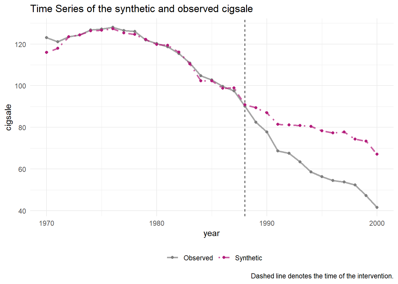

One can easily see that the post-propostion period is deviating downward. But to capture the actual quantitative differences between the observed and synthetic models, we can use plot_differences().

smoking_out %>% plot_differences()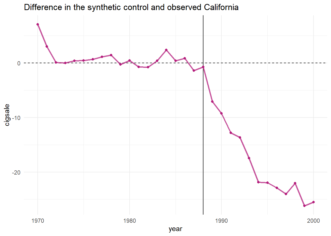

We might also want to know which (and how) units and variables were weighted by the model.

smoking_out %>% plot_weights()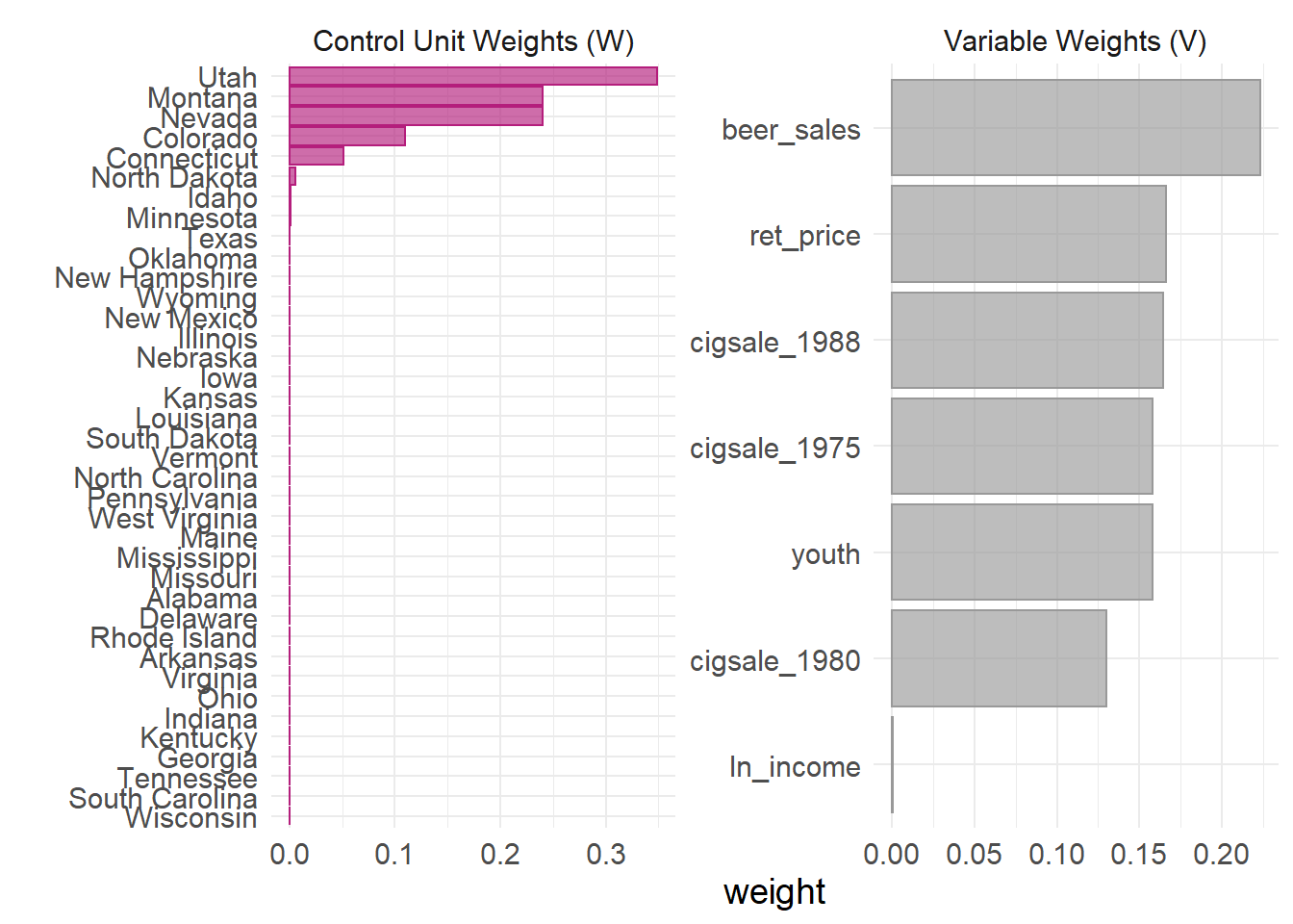

Smooth! The package also includes a host of grab_ functions to quickly retrieve parts of the tidy output. For example, a balance table can show us how comparable the synthetic control is to the observed covariates of the treated unit.

smoking_out %>% grab_balance_table()

## # A tibble: 7 x 4
##   variable     California synthetic_California donor_sample
##   <chr>             <dbl>                <dbl>        <dbl>
## 1 ln_income        10.1                  9.84         9.83 
## 2 ret_price        89.4                 89.4         87.3  
## 3 youth             0.174                0.174        0.173
## 4 beer_sales       24.3                 24.3         23.7  
## 5 cigsale_1975    127.                 127.         137.   
## 6 cigsale_1980    120.                 120.         138.   
## 7 cigsale_1988     90.1                 90.8        114.

Everything looks good there. One of the main uses for synthetic control models is for inference. In other words, can we infer causality for the somewhat dramatic change between the pre- and post-intervention periods? The package developer has included some very nice features to help with inference. From the package developer:

For inference, the method relies on repeating the method for every donor in the donor pool exactly as was done for the treated unit — i.e. generating placebo synthetic controls. By setting generate_placebos = TRUE when initializing the synth pipeline with synthetic_control(), placebo cases are automatically generated when constructing the synthetic control of interest. This makes it easy to explore how unique difference between the observed and synthetic unit is when compared to the placebos.

smoking_out %>% plot_placebos()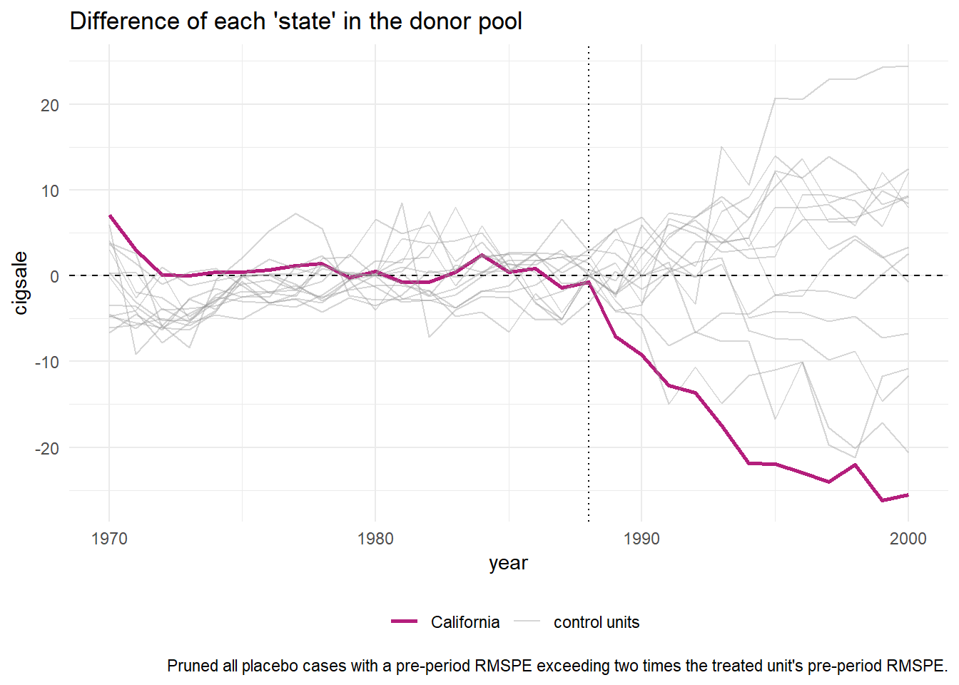

You might wonder why the plot above is only plotting a few of the donor cases. This is because the plain function of plot_placebos() automatically drops those cases where the data has a poor fit to the model. This is a fairly large difference between this package, which uses a frequentist approach, and BSTS, which obviously uses a Bayesian approach. Still, the package developer has a prune = FALSE argument you can use to see all the cases, regardless of data –> model fit.

Note that the plot_placebos() function automatically prunes any placebos that poorly fit the data in the pre-intervention period. The reason for doing so is purely visual: those units tend to throw off the scale when plotting the placebos. To prune, the function looks at the pre-intervention period mean squared prediction error (MSPE) (i.e. a metric that reflects how well the synthetic control maps to the observed outcome time series in pre-intervention period). If a placebo control has a MSPE that is two times beyond the target case (e.g. “California”), then it’s dropped. To turn off this behavior, set prune = FALSE.

smoking_out %>% plot_placebos(prune = FALSE)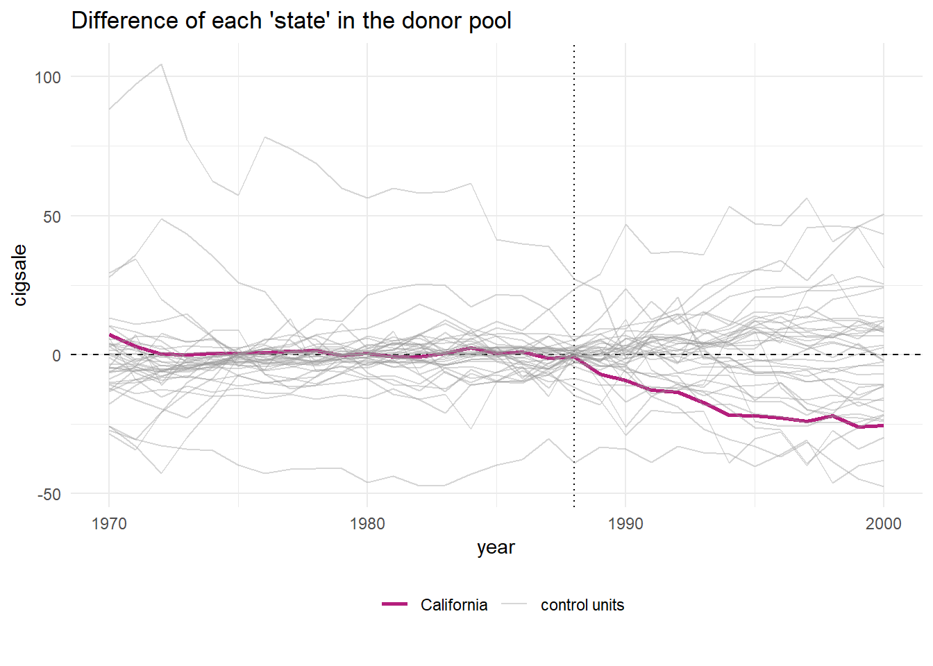

Some researchers prefer a frequentist approach, and one of the advantages of this approach is that we can derive Fisher’s Exact P-values based on work from Abadie et al., (2010). Interpretation is straightforward:

If the intervention had no effect, then the post-period and pre-period should continue to map onto one another fairly well, yielding a ratio close to 1. If the placebo units fit the data similarly, then we can’t reject the hull hypothesis that there is no effect brought about by the intervention.

This ratio can be easily plotted using plot_mspe_ratio(), offering insight into the rarity of the case where the intervention actually occurred.

smoking_out %>% plot_mspe_ratio()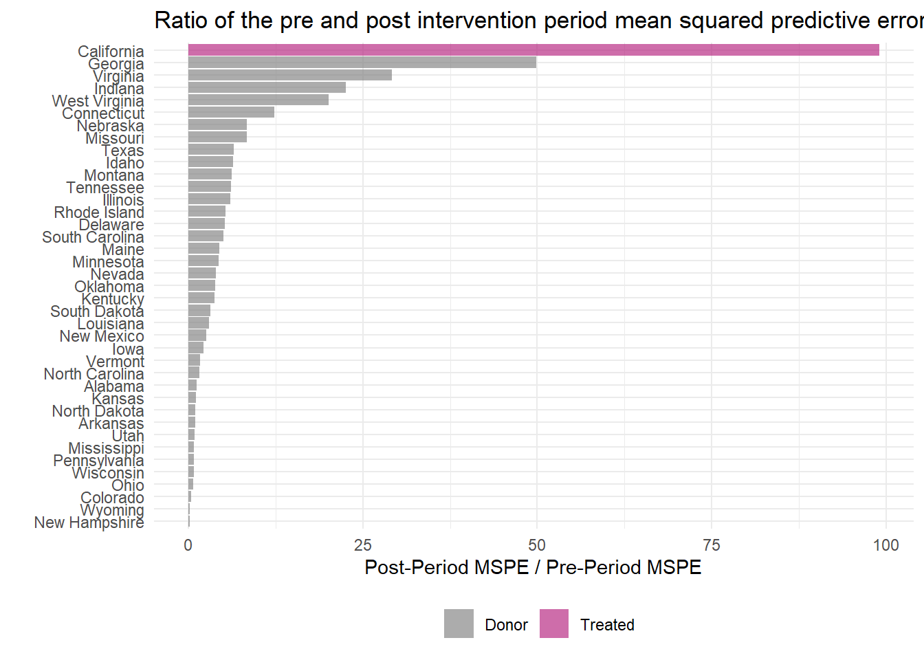

For those who want to publish their results, reviewers and readers are going to want a table of results. The tidysynth package has you covered.

smoking_out %>% grab_signficance()

## # A tibble: 39 x 8
##    unit_name  type  pre_mspe post_mspe mspe_ratio  rank fishers_exact_p~ z_score
##    <chr>      <chr>    <dbl>     <dbl>      <dbl> <int>            <dbl>   <dbl>
##  1 California Trea~     3.94     390.       99.0      1           0.0256  5.13  
##  2 Georgia    Donor     3.48     174.       49.8      2           0.0513  2.33  
##  3 Virginia   Donor     5.86     171.       29.2      3           0.0769  1.16  
##  4 Indiana    Donor    18.4      415.       22.6      4           0.103   0.787 
##  5 West Virg~ Donor    14.3      287.       20.1      5           0.128   0.646 
##  6 Connectic~ Donor    27.3      335.       12.3      6           0.154   0.202 
##  7 Nebraska   Donor     6.47      54.3       8.40     7           0.179  -0.0189
##  8 Missouri   Donor     9.19      77.0       8.38     8           0.205  -0.0199
##  9 Texas      Donor    24.5      160.        6.54     9           0.231  -0.125 
## 10 Idaho      Donor    53.2      340.        6.39    10           0.256  -0.133 
## # ... with 29 more rows

I really appreciate the work that’s gone into this package. It highlights the value of the tidyverse with human-readable code, and straightforward piping to make for very functional analysis with limited work. Great job to the developer!

I suggest reading further, as the package is apparently under active development. I also don’t go into the many grab_ functions that allow for the researcher to quickly “grab” elements of the model.

## # A tibble: 8 x 2
##   Function             Description                                              
##   <chr>                <chr>                                                    
## 1 grab_outcome()       Extract the outcome variable generated by synthetic_cont~
## 2 grab_predictors()    Extract the aggregate-level covariates generated by gene~
## 3 grab_unit_weights()  Extract the unit weights generated by generate_weights().
## 4 grab_predictor_weig~ Extract the predictor variable weights generated by gene~
## 5 grab_loss()          Extract the RMSE loss of the optimized weights generated~
## 6 grab_synthetic_cont~ Extract the synthetic control generated using generate_c~
## 7 grab_signficance()   Generate inferential statistics comparing the rarity of ~
## 8 grab_balance_table() Compare the distributions of the aggregate-level predict~