LEMAS 2016 and 2020 Turnover Comparison

Setup

First, let’s load the required libraries and set some global options for our code chunks. We will be using:

library(tidyverse)
library(readr)
library(here)
library(scales)
library(viridis)

Next, we will import the 2016 and 2020 LEMAS data and preprocess it, including cleaning column names and selecting relevant columns for our analysis. Make sure you have already imported the 2016 data to an object named df_raw_2016 and the 2020 data to one named df_raw_2020.

Data Import and Preprocessing

In this section, we will import the 2016 and 2020 LEMAS data, preprocess the data, and calculate the turnover rates.

## Import 2016 data

# Select relevant columns and calculate vacancies
df_2016 <- df_raw_2016 %>% select(
  lear_id,
  agencyname,
  agencytype,
  strata,
  population = popserved,
  ftsauth,
  ftsworn,
  total_separations = pers_sep_totr
) %>% mutate(vacancies = ftsauth - ftsworn) %>%
  filter(vacancies >= 0)

# Calculate vacancy and turnover rates
df_2016 <- df_2016 %>%
  mutate(vac_rate = (round((vacancies)/(ftsauth), digits = 2))*100,
         turnover_rate = total_separations / ftsworn)

# Filter agencies with 100 or more sworn officers
df100_2016 <- df_2016 %>% filter(strata == "(101) LP: 100+")

# Import 2020 data

# Renaming
df_2020 <- df_raw_2020 %>% select(
  agencyid,
  agencyname,
  agencytype = agencysamptype,
  strata,
  population = primarypop2020,
  sworn2019 = ftsworn_2019,
  sworn2020 = ftsworn,
  total_separations = tot_sep,
  vacancy2019 = ftvac_2019,
  vacancy2020 = ftvac
)


# Calculate vacancy rates
df_2020$vac_rate2020 <- (round((df_2020$vacancy2020)/(df_2020$sworn2020 + df_2020$vacancy2020), digits = 2))*100
df_2020$vac_rate2019 <- (round((df_2020$vacancy2019)/(df_2020$sworn2019 + df_2020$vacancy2019), digits = 2))*100

df_2020$turnover_rate <- df_2020$total_separations / df_2020$sworn2020

df100_2020 <- df_2020 %>% filter(sworn2019 > 99)

Turnover Rate Comparison

In this section, we will create a side-by-side comparison of the 2016 and 2020 turnover rates for local police agencies with 100 or more sworn officers.

First, we will filter out the outliers and calculate the mean and standard deviation for the turnover rates in both datasets.

df100_filtered_2016 <- df100_2016 %>% 
  filter(turnover_rate <= 0.30)

turnover_mean_2016 <- mean(df100_filtered_2016$turnover_rate, na.rm = TRUE)
turnover_sd_2016 <- sd(df100_filtered_2016$turnover_rate, na.rm = TRUE)

df100_filtered_2020 <- df100_2020 %>% 
  filter(turnover_rate <= 0.30)

turnover_mean_2020 <- mean(df100_filtered_2020$turnover_rate, na.rm = TRUE)
turnover_sd_2020 <- sd(df100_filtered_2020$turnover_rate, na.rm = TRUE)

Next, let’s create a reusable function to generate the turnover rate plots for both years.

plot_turnover <- function(df, year, mean, sd) {
  ggplot(data = df, aes(x = turnover_rate)) +  # Create the base ggplot with turnover_rate on the x-axis
    geom_histogram(binwidth = 0.025, fill = "steelblue", color = "white") +  # Add a histogram with custom colors and binwidth
    scale_x_continuous(breaks = seq(0, 0.5, 0.02), labels = scales::percent) +  # Set x-axis breaks and labels
    labs(title = paste0(year, " Turnover Rate"),  # Set the title
         subtitle = paste0("Local Police Agencies with 100+ Sworn Officers (n=", nrow(df), ")\n",
                           "Mean: ", scales::percent(mean, accuracy = 0.01), " | ",
                           "SD: ", scales::percent(sd, accuracy = 0.01)),  # Set the subtitle with mean and SD values
         x = "Turnover Rate",  # Set the x-axis label
         y = "Frequency") +  # Set the y-axis label
    geom_vline(xintercept = mean, linetype="dashed", linewidth = 1.5, color = "yellow") +  # Add a vertical dashed line at the mean
    theme_minimal() +  # Apply the minimal theme
    theme(plot.title = element_text(size = 18, face = "bold", margin = margin(10, 0, 5, 0)),
          plot.subtitle = element_text(size = 14, margin = margin(0, 0, 10, 0)),
          axis.title = element_text(size = 14, face = "bold"),
          axis.text = element_text(size = 12),
          panel.grid.major.y = element_line(color = "gray", linetype = "dashed"))  # Customize theme elements
}

Using the plot_turnover function, let’s create the turnover rate plots for 2016 and 2020.

plot_2016 <- plot_turnover(df100_filtered_2016, "2016", turnover_mean_2016, turnover_sd_2016)
plot_2020 <- plot_turnover(df100_filtered_2020, "2020", turnover_mean_2020, turnover_sd_2020)

Finally, let’s display the plots side-by-side to compare the turnover rates in 2016 and 2020

plot_2016
plot_2020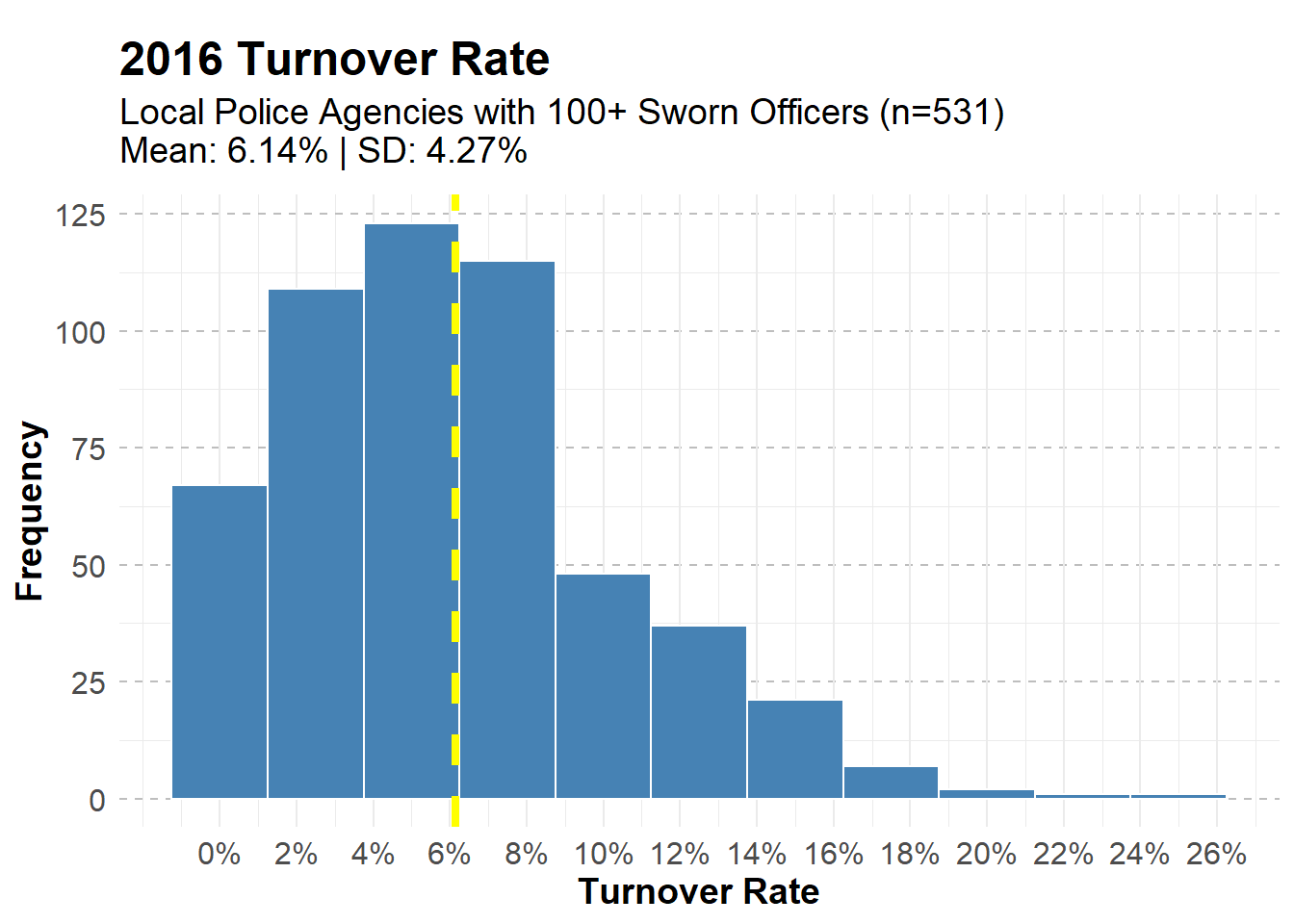

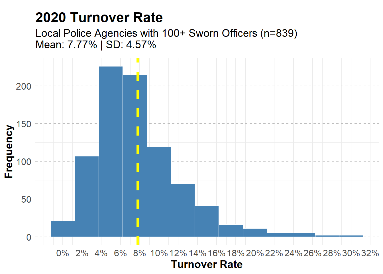
From the side-by-side comparison, we can observe the differences in turnover rates between 2016 and 2020 for local police agencies with 100 or more sworn officers. Note the distribution of the turnover rates and how the mean and standard deviation have changed over time.

Conclusion

In this blog post, I have demonstrated how to import, preprocess, and visualize the LEMAS 2016 and 2020 datasets to analyze and compare the turnover rates in local police agencies with 100 or more sworn officers. The side-by-side comparison of the turnover rates provides valuable insights into the changes within law enforcement agencies over the years.

By following these steps, you can further explore and analyze the LEMAS data and draw conclusions about various aspects of law enforcement management and administration.

Feel free to extend this analysis to other variables or subsets of agencies within the LEMAS data or even compare other years to gain a deeper understanding of trends in law enforcement. Happy analyzing!