Tidying STM with tidytext
Libraries
library(tidytext)
library(ggthemes)
library(tidyverse)
library(ggplot2)
library(dplyr)
library(scales)
Load Previous STM Objects
I have previously run stm models for topics ranging from 3 to 25. Based on the fit indices, a six-topic model was selected. I am not showing that analysis here, but instead loading the saved stm objects (the model and the ‘out’ object).
Tidy the stm model
I am using the tidytext package from Julia Silge, which she demonstrates in a blog post here.
td_beta <- tidy(modelfit6)
td_beta
## # A tibble: 1,416 x 3
## topic term beta
## <int> <chr> <dbl>
## 1 1 abil 9.13e-61
## 2 2 abil 6.07e-55
## 3 3 abil 1.51e- 2
## 4 4 abil 2.98e-54
## 5 5 abil 3.66e-63
## 6 6 abil 2.39e-58
## 7 1 account 1.57e-91
## 8 2 account 1.37e-25
## 9 3 account 4.28e-66
## 10 4 account 6.47e-63
## # ... with 1,406 more rowstd_gamma <- tidy(modelfit6, matrix = "gamma",
document_names = rownames(out$meta))
td_gamma## # A tibble: 1,266 x 3
## document topic gamma
## <chr> <int> <dbl>
## 1 1 1 0.00343
## 2 2 1 0.00462
## 3 3 1 0.0861
## 4 4 1 0.0467
## 5 5 1 0.0106
## 6 6 1 0.00306
## 7 7 1 0.00419
## 8 8 1 0.0511
## 9 9 1 0.00356
## 10 10 1 0.144
## # ... with 1,256 more rowsPlot Topic Relevance
top_terms <- td_beta %>%
  arrange(beta) %>%
  group_by(topic) %>%
  top_n(7, beta) %>%
  arrange(-beta) %>%
  select(topic, term) %>%
  summarise(terms = list(term)) %>%
  mutate(terms = map(terms, paste, collapse = ", ")) %>%
  unnest()

gamma_terms <- td_gamma %>%
  group_by(topic) %>%
  summarise(gamma = mean(gamma)) %>%
  arrange(desc(gamma)) %>%
  left_join(top_terms, by = "topic") %>%
  mutate(topic = paste0("Topic ", topic),
         topic = reorder(topic, gamma))

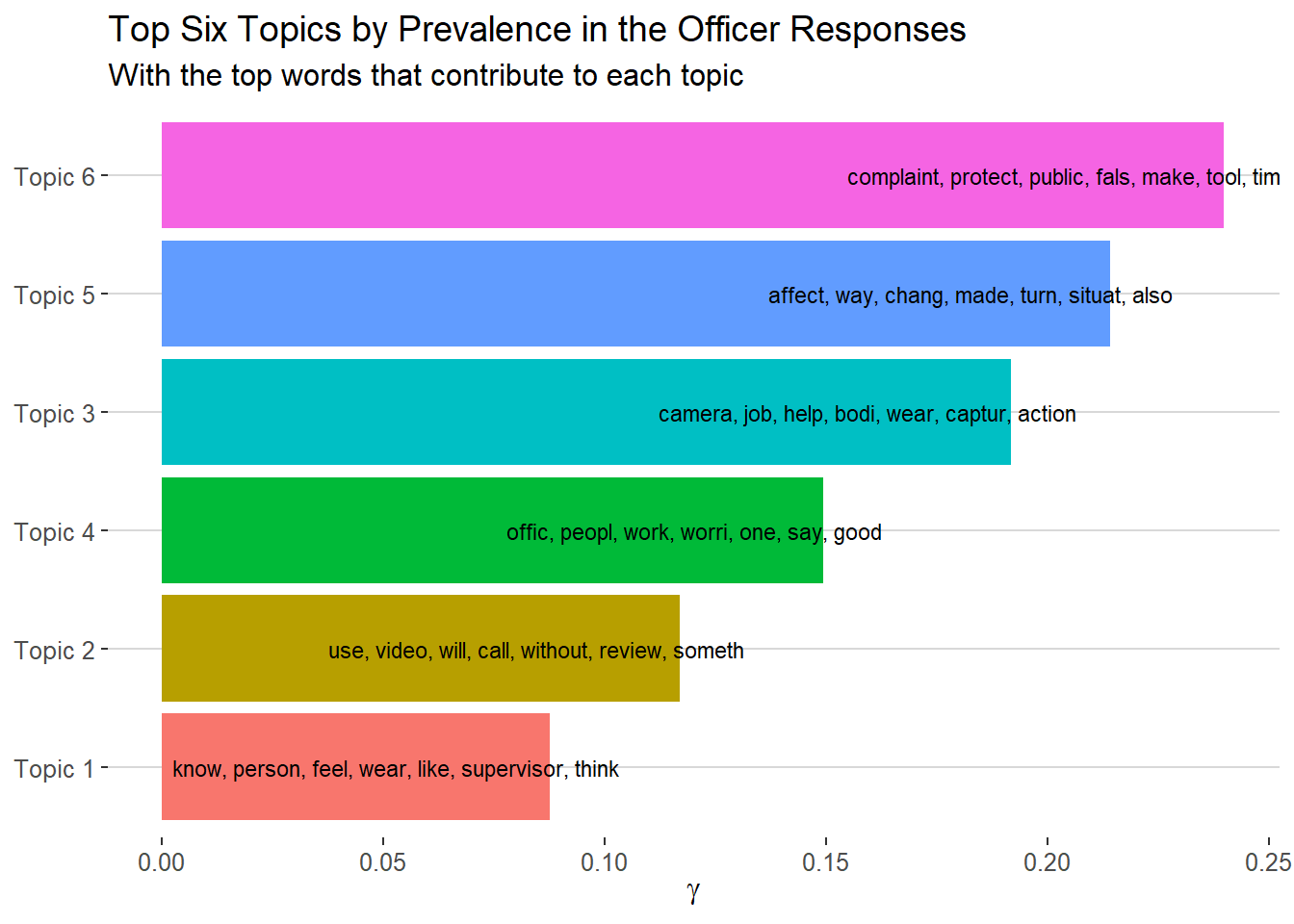
gamma_terms %>%
  top_n(6, gamma) %>%
  ggplot(aes(topic, gamma, label = terms, fill = topic)) +
  geom_col(show.legend = FALSE) +
  geom_text(hjust = 0.85, nudge_y = 0.0005, size = 3) +
  coord_flip() +
  theme_hc() +
  theme(plot.title = element_text(size = 14)) +
  labs(x = NULL, y = expression(gamma),
       title = "Top Six Topics by Prevalence in the Officer Responses",
       subtitle = "With the top words that contribute to each topic")
Table of Topic Proportions with Top Terms
require(knitr)
gamma_terms %>%
  select(topic, gamma, terms) %>%
  kable(digits = 3,
col.names = c("Topic", "Expected topic proportion", "Top 6 terms"))| Topic | Expected topic proportion | Top 6 terms |
|---|---|---|
| Topic 6 | 0.240 | complaint, protect, public, fals, make, tool, time |
| Topic 5 | 0.214 | affect, way, chang, made, turn, situat, also |
| Topic 3 | 0.192 | camera, job, help, bodi, wear, captur, action |
| Topic 4 | 0.149 | offic, peopl, work, worri, one, say, good |
| Topic 2 | 0.117 | use, video, will, call, without, review, someth |
| Topic 1 | 0.088 | know, person, feel, wear, like, supervisor, think |