Week 10 Solutions
So you want to be a data scientist
This week can feel like a bit of a doozy, as the difficulty really ramps up. Something to remember - most data scientists spend most of their time cleaning, transforming, and tidying their data. That’s what these chapters and questions are all about. So I want to make sure you have the correct answers, but more importantly, I want you to know you are not alone, this stuff is hard! I’ve put the quote in front of you before, but this little bit of wisdom from Hadley Wickham, lead author of our class textbook, is important during times like we’re having right now:
“There is no way of going from knowing nothing about a subject to knowing something about a subject without going through a period of much frustration and suckiness. Push through. You’ll suck less.”
Now, onto the answers!
Exercise 5.2.4
Why is
NA ^ 0not missing? Why isNA | TRUEnot missing? Why isFALSE & NAnot missing? Can you figure out the general rule? (NA * 0is a tricky counterexample!)
NA ^ 0## [1] 1NA ^ 0 == 1 since for all numeric values \(x ^ 0 = 1\).
NA | TRUE## [1] TRUENA | TRUE is TRUE because anything or TRUE is TRUE.
If the missing value were TRUE, then TRUE | TRUE == TRUE,
and if the missing value was FALSE, then FALSE | TRUE == TRUE.
NA & FALSE## [1] FALSEThe value of NA & FALSE is FALSE because anything and FALSE is always FALSE.
If the missing value were TRUE, then TRUE & FALSE == FALSE,
and if the missing value was FALSE, then FALSE & FALSE == FALSE.
NA | FALSE## [1] NAFor NA | FALSE, the value is unknown since TRUE | FALSE == TRUE, but FALSE | FALSE == FALSE.
NA & TRUE## [1] NAFor NA & TRUE, the value is unknown since FALSE & TRUE== FALSE, but TRUE & TRUE == TRUE.
NA * 0## [1] NASince \(x * 0 = 0\) for all finite numbers we might expect NA * 0 == 0, but that’s not the case.
The reason that NA * 0 != 0 is that \(0 \times \infty\) and \(0 \times -\infty\) are undefined.
R represents undefined results as NaN, which is an abbreviation of “not a number”.
Inf * 0## [1] NaN-Inf * 0## [1] NaNExercise 5.3.1
How could you use
arrange()to sort all missing values to the start? (Hint: useis.na()).
The arrange() function puts NA values last.
arrange(flights, dep_time) %>%
  tail()
## # A tibble: 6 x 19
## year month day dep_time sched_dep_time dep_delay arr_time sched_arr_time
## <int> <int> <int> <int> <int> <dbl> <int> <int>
## 1 2013 9 30 NA 1842 NA NA 2019
## 2 2013 9 30 NA 1455 NA NA 1634
## 3 2013 9 30 NA 2200 NA NA 2312
## 4 2013 9 30 NA 1210 NA NA 1330
## 5 2013 9 30 NA 1159 NA NA 1344
## 6 2013 9 30 NA 840 NA NA 1020
## # ... with 11 more variables: arr_delay <dbl>, carrier <chr>, flight <int>,
## # tailnum <chr>, origin <chr>, dest <chr>, air_time <dbl>, distance <dbl>,
## # hour <dbl>, minute <dbl>, time_hour <dttm>Using desc() does not change that.
arrange(flights, desc(dep_time))## # A tibble: 336,776 x 19
## year month day dep_time sched_dep_time dep_delay arr_time sched_arr_time
## <int> <int> <int> <int> <int> <dbl> <int> <int>
## 1 2013 10 30 2400 2359 1 327 337
## 2 2013 11 27 2400 2359 1 515 445
## 3 2013 12 5 2400 2359 1 427 440
## 4 2013 12 9 2400 2359 1 432 440
## 5 2013 12 9 2400 2250 70 59 2356
## 6 2013 12 13 2400 2359 1 432 440
## 7 2013 12 19 2400 2359 1 434 440
## 8 2013 12 29 2400 1700 420 302 2025
## 9 2013 2 7 2400 2359 1 432 436
## 10 2013 2 7 2400 2359 1 443 444
## # ... with 336,766 more rows, and 11 more variables: arr_delay <dbl>,
## # carrier <chr>, flight <int>, tailnum <chr>, origin <chr>, dest <chr>,
## # air_time <dbl>, distance <dbl>, hour <dbl>, minute <dbl>, time_hour <dttm>To put NA values first, we can add an indicator of whether the column has a missing value.
Then we sort by the missing indicator column and the column of interest.
For example, to sort the data frame by departure time (dep_time) in ascending order but NA values first, run the following.
arrange(flights, desc(is.na(dep_time)), dep_time)## # A tibble: 336,776 x 19
## year month day dep_time sched_dep_time dep_delay arr_time sched_arr_time
## <int> <int> <int> <int> <int> <dbl> <int> <int>
## 1 2013 1 1 NA 1630 NA NA 1815
## 2 2013 1 1 NA 1935 NA NA 2240
## 3 2013 1 1 NA 1500 NA NA 1825
## 4 2013 1 1 NA 600 NA NA 901
## 5 2013 1 2 NA 1540 NA NA 1747
## 6 2013 1 2 NA 1620 NA NA 1746
## 7 2013 1 2 NA 1355 NA NA 1459
## 8 2013 1 2 NA 1420 NA NA 1644
## 9 2013 1 2 NA 1321 NA NA 1536
## 10 2013 1 2 NA 1545 NA NA 1910
## # ... with 336,766 more rows, and 11 more variables: arr_delay <dbl>,
## # carrier <chr>, flight <int>, tailnum <chr>, origin <chr>, dest <chr>,
## # air_time <dbl>, distance <dbl>, hour <dbl>, minute <dbl>, time_hour <dttm>The flights will first be sorted by desc(is.na(dep_time)).
Since desc(is.na(dep_time)) is either TRUE when dep_time is missing, or FALSE, when it is not, the rows with missing values of dep_time will come first, since TRUE > FALSE.
Exercise 5.4.1
Brainstorm as many ways as possible to select
dep_time,dep_delay,arr_time, andarr_delayfrom flights.
These are a few ways to select columns.
Specify columns names as unquoted variable names.
select(flights, dep_time, dep_delay, arr_time, arr_delay)## # A tibble: 336,776 x 4 ## dep_time dep_delay arr_time arr_delay ## <int> <dbl> <int> <dbl> ## 1 517 2 830 11 ## 2 533 4 850 20 ## 3 542 2 923 33 ## 4 544 -1 1004 -18 ## 5 554 -6 812 -25 ## 6 554 -4 740 12 ## 7 555 -5 913 19 ## 8 557 -3 709 -14 ## 9 557 -3 838 -8 ## 10 558 -2 753 8 ## # ... with 336,766 more rowsSpecify column names as strings.
select(flights, "dep_time", "dep_delay", "arr_time", "arr_delay")## # A tibble: 336,776 x 4 ## dep_time dep_delay arr_time arr_delay ## <int> <dbl> <int> <dbl> ## 1 517 2 830 11 ## 2 533 4 850 20 ## 3 542 2 923 33 ## 4 544 -1 1004 -18 ## 5 554 -6 812 -25 ## 6 554 -4 740 12 ## 7 555 -5 913 19 ## 8 557 -3 709 -14 ## 9 557 -3 838 -8 ## 10 558 -2 753 8 ## # ... with 336,766 more rowsSpecify the column numbers of the variables.
select(flights, 4, 6, 7, 9)## # A tibble: 336,776 x 4 ## dep_time dep_delay arr_time arr_delay ## <int> <dbl> <int> <dbl> ## 1 517 2 830 11 ## 2 533 4 850 20 ## 3 542 2 923 33 ## 4 544 -1 1004 -18 ## 5 554 -6 812 -25 ## 6 554 -4 740 12 ## 7 555 -5 913 19 ## 8 557 -3 709 -14 ## 9 557 -3 838 -8 ## 10 558 -2 753 8 ## # ... with 336,766 more rowsThis works, but is not good practice for two reasons. First, the column location of variables may change, resulting in code that may continue to run without error, but produce the wrong answer. Second code is obfuscated, since it is not clear from the code which variables are being selected. What variable does column 6 correspond to? I just wrote the code, and I’ve already forgotten.
Specify the names of the variables with character vector and
any_of()orall_of()select(flights, all_of(c("dep_time", "dep_delay", "arr_time", "arr_delay")))## # A tibble: 336,776 x 4 ## dep_time dep_delay arr_time arr_delay ## <int> <dbl> <int> <dbl> ## 1 517 2 830 11 ## 2 533 4 850 20 ## 3 542 2 923 33 ## 4 544 -1 1004 -18 ## 5 554 -6 812 -25 ## 6 554 -4 740 12 ## 7 555 -5 913 19 ## 8 557 -3 709 -14 ## 9 557 -3 838 -8 ## 10 558 -2 753 8 ## # ... with 336,766 more rowsselect(flights, any_of(c("dep_time", "dep_delay", "arr_time", "arr_delay")))## # A tibble: 336,776 x 4 ## dep_time dep_delay arr_time arr_delay ## <int> <dbl> <int> <dbl> ## 1 517 2 830 11 ## 2 533 4 850 20 ## 3 542 2 923 33 ## 4 544 -1 1004 -18 ## 5 554 -6 812 -25 ## 6 554 -4 740 12 ## 7 555 -5 913 19 ## 8 557 -3 709 -14 ## 9 557 -3 838 -8 ## 10 558 -2 753 8 ## # ... with 336,766 more rowsThis is useful because the names of the variables can be stored in a variable and passed to
all_of()orany_of().variables <- c("dep_time", "dep_delay", "arr_time", "arr_delay") select(flights, all_of(variables))## # A tibble: 336,776 x 4 ## dep_time dep_delay arr_time arr_delay ## <int> <dbl> <int> <dbl> ## 1 517 2 830 11 ## 2 533 4 850 20 ## 3 542 2 923 33 ## 4 544 -1 1004 -18 ## 5 554 -6 812 -25 ## 6 554 -4 740 12 ## 7 555 -5 913 19 ## 8 557 -3 709 -14 ## 9 557 -3 838 -8 ## 10 558 -2 753 8 ## # ... with 336,766 more rowsThese two functions replace the deprecated function
one_of().Selecting the variables by matching the start of their names using
starts_with().select(flights, starts_with("dep_"), starts_with("arr_"))## # A tibble: 336,776 x 4 ## dep_time dep_delay arr_time arr_delay ## <int> <dbl> <int> <dbl> ## 1 517 2 830 11 ## 2 533 4 850 20 ## 3 542 2 923 33 ## 4 544 -1 1004 -18 ## 5 554 -6 812 -25 ## 6 554 -4 740 12 ## 7 555 -5 913 19 ## 8 557 -3 709 -14 ## 9 557 -3 838 -8 ## 10 558 -2 753 8 ## # ... with 336,766 more rowsSelecting the variables using regular expressions with
matches(). Regular expressions provide a flexible way to match string patterns and are discussed in the Strings chapter.select(flights, matches("^(dep|arr)_(time|delay)$"))## # A tibble: 336,776 x 4 ## dep_time dep_delay arr_time arr_delay ## <int> <dbl> <int> <dbl> ## 1 517 2 830 11 ## 2 533 4 850 20 ## 3 542 2 923 33 ## 4 544 -1 1004 -18 ## 5 554 -6 812 -25 ## 6 554 -4 740 12 ## 7 555 -5 913 19 ## 8 557 -3 709 -14 ## 9 557 -3 838 -8 ## 10 558 -2 753 8 ## # ... with 336,766 more rowsSpecify the names of the variables with a character vector and use the bang-bang operator (
!!).variables <- c("dep_time", "dep_delay", "arr_time", "arr_delay") select(flights, !!variables)## # A tibble: 336,776 x 4 ## dep_time dep_delay arr_time arr_delay ## <int> <dbl> <int> <dbl> ## 1 517 2 830 11 ## 2 533 4 850 20 ## 3 542 2 923 33 ## 4 544 -1 1004 -18 ## 5 554 -6 812 -25 ## 6 554 -4 740 12 ## 7 555 -5 913 19 ## 8 557 -3 709 -14 ## 9 557 -3 838 -8 ## 10 558 -2 753 8 ## # ... with 336,766 more rowsThis and the following answers use the features of tidy evaluation not covered in R4DS but covered in the Programming with dplyr vignette.
Specify the names of the variables in a character or list vector and use the bang-bang-bang operator.
variables <- c("dep_time", "dep_delay", "arr_time", "arr_delay")
select(flights, !!!variables)
## # A tibble: 336,776 x 4 ## dep_time dep_delay arr_time arr_delay ## <int> <dbl> <int> <dbl> ## 1 517 2 830 11 ## 2 533 4 850 20 ## 3 542 2 923 33 ## 4 544 -1 1004 -18 ## 5 554 -6 812 -25 ## 6 554 -4 740 12 ## 7 555 -5 913 19 ## 8 557 -3 709 -14 ## 9 557 -3 838 -8 ## 10 558 -2 753 8 ## # ... with 336,766 more rowsSpecify the unquoted names of the variables in a list using
syms()and use the bang-bang-bang operator.variables <- syms(c("dep_time", "dep_delay", "arr_time", "arr_delay")) select(flights, !!!variables)## # A tibble: 336,776 x 4 ## dep_time dep_delay arr_time arr_delay ## <int> <dbl> <int> <dbl> ## 1 517 2 830 11 ## 2 533 4 850 20 ## 3 542 2 923 33 ## 4 544 -1 1004 -18 ## 5 554 -6 812 -25 ## 6 554 -4 740 12 ## 7 555 -5 913 19 ## 8 557 -3 709 -14 ## 9 557 -3 838 -8 ## 10 558 -2 753 8 ## # ... with 336,766 more rows
Some things that don’t work are:
Matching the ends of their names using
ends_with()since this will incorrectly include other variables. For example,select(flights, ends_with("arr_time"), ends_with("dep_time"))## # A tibble: 336,776 x 4 ## arr_time sched_arr_time dep_time sched_dep_time ## <int> <int> <int> <int> ## 1 830 819 517 515 ## 2 850 830 533 529 ## 3 923 850 542 540 ## 4 1004 1022 544 545 ## 5 812 837 554 600 ## 6 740 728 554 558 ## 7 913 854 555 600 ## 8 709 723 557 600 ## 9 838 846 557 600 ## 10 753 745 558 600 ## # ... with 336,766 more rowsMatching the names using
contains()since there is not a pattern that can include all these variables without incorrectly including others.select(flights, contains("_time"), contains("arr_"))## # A tibble: 336,776 x 6 ## dep_time sched_dep_time arr_time sched_arr_time air_time arr_delay ## <int> <int> <int> <int> <dbl> <dbl> ## 1 517 515 830 819 227 11 ## 2 533 529 850 830 227 20 ## 3 542 540 923 850 160 33 ## 4 544 545 1004 1022 183 -18 ## 5 554 600 812 837 116 -25 ## 6 554 558 740 728 150 12 ## 7 555 600 913 854 158 19 ## 8 557 600 709 723 53 -14 ## 9 557 600 838 846 140 -8 ## 10 558 600 753 745 138 8 ## # ... with 336,766 more rows
Exercise 5.5.2
Compare
air_timewitharr_time - dep_time. What do you expect to see? What do you see? What do you need to do to fix it?
I expect that air_time is the difference between the arrival (arr_time) and departure times (dep_time).
In other words, air_time = arr_time - dep_time.
To check that this relationship, I’ll first need to convert the times to a form more amenable to arithmetic operations using the same calculations as the previous exercise.
flights_airtime <-
  mutate(flights,
    dep_time = (dep_time %/% 100 * 60 + dep_time %% 100) %% 1440,
    arr_time = (arr_time %/% 100 * 60 + arr_time %% 100) %% 1440,
    air_time_diff = air_time - arr_time + dep_time
  )
So, does air_time = arr_time - dep_time?
If so, there should be no flights with non-zero values of air_time_diff.
nrow(filter(flights_airtime, air_time_diff != 0))## [1] 327150It turns out that there are many flights for which air_time != arr_time - dep_time.
Other than data errors, I can think of two reasons why air_time would not equal arr_time - dep_time.
The flight passes midnight, so
arr_time < dep_time. In these cases, the difference in airtime should be by 24 hours (1,440 minutes).The flight crosses time zones, and the total air time will be off by hours (multiples of 60). All flights in
flightsdeparted from New York City and are domestic flights in the US. This means that flights will all be to the same or more westerly time zones. Given the time-zones in the US, the differences due to time-zone should be 60 minutes (Central) 120 minutes (Mountain), 180 minutes (Pacific), 240 minutes (Alaska), or 300 minutes (Hawaii).
Both of these explanations have clear patterns that I would expect to see if they
were true.
In particular, in both cases, since time-zones and crossing midnight only affects the hour part of the time, all values of air_time_diff should be divisible by 60.
I’ll visually check this hypothesis by plotting the distribution of air_time_diff.
If those two explanations are correct, distribution of air_time_diff should comprise only spikes at multiples of 60.
ggplot(flights_airtime, aes(x = air_time_diff)) +
  geom_histogram(binwidth = 1)
## Warning: Removed 9430 rows containing non-finite values (stat_bin).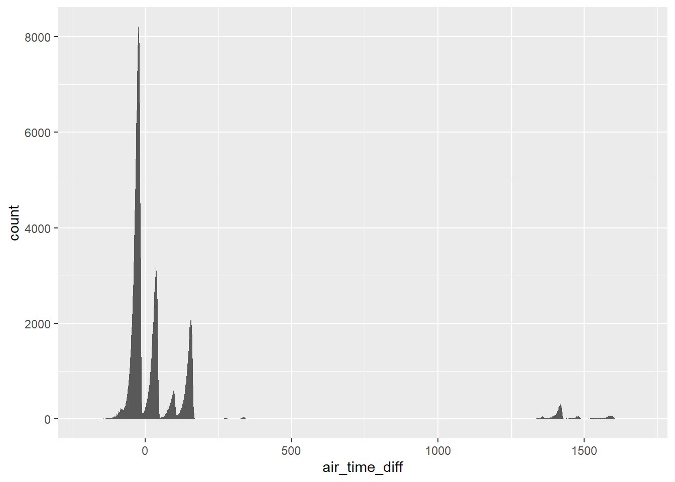 This is not the case.
While, the distribution of
This is not the case.
While, the distribution of air_time_diff has modes at multiples of 60 as hypothesized,
it shows that there are many flights in which the difference between air time and local arrival and departure times is not divisible by 60.
Let’s also look at flights with Los Angeles as a destination. The discrepancy should be 180 minutes.
ggplot(filter(flights_airtime, dest == "LAX"), aes(x = air_time_diff)) +
  geom_histogram(binwidth = 1)
## Warning: Removed 148 rows containing non-finite values (stat_bin).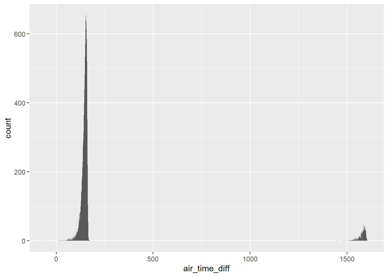
To fix these time-zone issues, I would want to convert all the times to a date-time to handle overnight flights, and from local time to a common time zone, most likely UTC, to handle flights crossing time-zones.
The tzone column of nycflights13::airports gives the time-zone of each airport.
See the “Dates and Times” for an introduction on working with date and time data.
But that still leaves the other differences unexplained.
So what else might be going on?
There seem to be too many problems for this to be data entry problems, so I’m probably missing something.
So, I’ll reread the documentation to make sure that I understand the definitions of arr_time, dep_time, and
air_time.
The documentation contains a link to the source of the flights data, https://www.transtats.bts.gov/DL_SelectFields.asp?Table_ID=236.
This documentation shows that the flights data does not contain the variables TaxiIn, TaxiOff, WheelsIn, and WheelsOff.
It appears that the air_time variable refers to flight time, which is defined as the time between wheels-off (take-off) and wheels-in (landing).
But the flight time does not include time spent on the runway taxiing to and from gates.
With this new understanding of the data, I now know that the relationship between air_time, arr_time, and dep_time is air_time <= arr_time - dep_time, supposing that the time zones of arr_time and dep_time are in the same time zone.
Exercise 5.6.7
Brainstorm at least 5 different ways to assess the typical delay characteristics of a group of flights. Consider the following scenarios:
- A flight is 15 minutes early 50% of the time, and 15 minutes late 50% of the time.
- A flight is always 10 minutes late.
- A flight is 30 minutes early 50% of the time, and 30 minutes late 50% of the time.
- 99% of the time a flight is on time. 1% of the time it’s 2 hours late.
Which is more important: arrival delay or departure delay?
What this question gets at is a fundamental question of data analysis: the cost function. As analysts, the reason we are interested in flight delay because it is costly to passengers. But it is worth thinking carefully about how it is costly and use that information in ranking and measuring these scenarios.
In many scenarios, arrival delay is more important.
In most cases, being arriving late is more costly to the passenger since it could disrupt the next stages of their travel, such as connecting flights or scheduled meetings.
If a departure is delayed without affecting the arrival time, this delay will not have those affects plans nor does it affect the total time spent traveling.
This delay could be beneficial, if less time is spent in the cramped confines of the airplane itself, or a negative, if that delayed time is still spent in the cramped confines of the airplane on the runway.
Variation in arrival time is worse than consistency. If a flight is always 30 minutes late and that delay is known, then it is as if the arrival time is that delayed time. The traveler could easily plan for this. But higher variation in flight times makes it harder to plan.
5.6.7.2
Come up with another approach that will give you the same output as
not_cancelled %>% count(dest)andnot_cancelled %>% count(tailnum, wt = distance)(without usingcount()).
not_cancelled <- flights %>%
  filter(!is.na(dep_delay), !is.na(arr_delay))
The first expression is the following.
not_cancelled %>%
  count(dest)
## # A tibble: 104 x 2
## dest n
## <chr> <int>
## 1 ABQ 254
## 2 ACK 264
## 3 ALB 418
## 4 ANC 8
## 5 ATL 16837
## 6 AUS 2411
## 7 AVL 261
## 8 BDL 412
## 9 BGR 358
## 10 BHM 269
## # ... with 94 more rowsThe count() function counts the number of instances within each group of variables.
Instead of using the count() function, we can combine the group_by() and summarise() verbs.
not_cancelled %>%
  group_by(dest) %>%
  summarise(n = length(dest))
## # A tibble: 104 x 2
## dest n
## <chr> <int>
## 1 ABQ 254
## 2 ACK 264
## 3 ALB 418
## 4 ANC 8
## 5 ATL 16837
## 6 AUS 2411
## 7 AVL 261
## 8 BDL 412
## 9 BGR 358
## 10 BHM 269
## # ... with 94 more rowsAn alternative method for getting the number of observations in a data frame is the function n().
not_cancelled %>%
  group_by(dest) %>%
  summarise(n = n())
## # A tibble: 104 x 2
## dest n
## <chr> <int>
## 1 ABQ 254
## 2 ACK 264
## 3 ALB 418
## 4 ANC 8
## 5 ATL 16837
## 6 AUS 2411
## 7 AVL 261
## 8 BDL 412
## 9 BGR 358
## 10 BHM 269
## # ... with 94 more rowsAnother alternative to count() is to use group_by() followed by tally().
In fact, count() is effectively a short-cut for group_by() followed by tally().
not_cancelled %>%
  group_by(tailnum) %>%
  tally()
## # A tibble: 4,037 x 2
## tailnum n
## <chr> <int>
## 1 D942DN 4
## 2 N0EGMQ 352
## 3 N10156 145
## 4 N102UW 48
## 5 N103US 46
## 6 N104UW 46
## 7 N10575 269
## 8 N105UW 45
## 9 N107US 41
## 10 N108UW 60
## # ... with 4,027 more rowsThe second expression also uses the count() function, but adds a wt argument.
not_cancelled %>%
  count(tailnum, wt = distance)
## # A tibble: 4,037 x 2
## tailnum n
## <chr> <dbl>
## 1 D942DN 3418
## 2 N0EGMQ 239143
## 3 N10156 109664
## 4 N102UW 25722
## 5 N103US 24619
## 6 N104UW 24616
## 7 N10575 139903
## 8 N105UW 23618
## 9 N107US 21677
## 10 N108UW 32070
## # ... with 4,027 more rowsAs before, we can replicate count() by combining the group_by() and summarise() verbs.
But this time instead of using length(), we will use sum() with the weighting variable.
not_cancelled %>%
  group_by(tailnum) %>%
  summarise(n = sum(distance))
## # A tibble: 4,037 x 2
## tailnum n
## <chr> <dbl>
## 1 D942DN 3418
## 2 N0EGMQ 239143
## 3 N10156 109664
## 4 N102UW 25722
## 5 N103US 24619
## 6 N104UW 24616
## 7 N10575 139903
## 8 N105UW 23618
## 9 N107US 21677
## 10 N108UW 32070
## # ... with 4,027 more rowsLike the previous example, we can also use the combination group_by() and tally().
Any arguments to tally() are summed.
not_cancelled %>%
  group_by(tailnum) %>%
  tally(distance)
## # A tibble: 4,037 x 2
## tailnum n
## <chr> <dbl>
## 1 D942DN 3418
## 2 N0EGMQ 239143
## 3 N10156 109664
## 4 N102UW 25722
## 5 N103US 24619
## 6 N104UW 24616
## 7 N10575 139903
## 8 N105UW 23618
## 9 N107US 21677
## 10 N108UW 32070
## # ... with 4,027 more rows5.6.7.3
Our definition of cancelled flights
(is.na(dep_delay) | is.na(arr_delay))is slightly suboptimal. Why? Which is the most important column?
If a flight never departs, then it won’t arrive.
A flight could also depart and not arrive if it crashes, or if it is redirected and lands in an airport other than its intended destination.
So the most important column is arr_delay, which indicates the amount of delay in arrival.
filter(flights, !is.na(dep_delay), is.na(arr_delay)) %>%
  select(dep_time, arr_time, sched_arr_time, dep_delay, arr_delay)
## # A tibble: 1,175 x 5
## dep_time arr_time sched_arr_time dep_delay arr_delay
## <int> <int> <int> <dbl> <dbl>
## 1 1525 1934 1805 -5 NA
## 2 1528 2002 1647 29 NA
## 3 1740 2158 2020 -5 NA
## 4 1807 2251 2103 29 NA
## 5 1939 29 2151 59 NA
## 6 1952 2358 2207 22 NA
## 7 2016 NA 2220 46 NA
## 8 905 1313 1045 43 NA
## 9 1125 1445 1146 120 NA
## 10 1848 2333 2151 8 NA
## # ... with 1,165 more rowsIn this data dep_time can be non-missing and arr_delay missing but arr_time not missing.
Some further research found that these rows correspond to diverted flights.
The BTS database that is the source for the flights table contains additional information for diverted flights that is not included in the nycflights13 data.
The source contains a column DivArrDelay with the description:
Difference in minutes between scheduled and actual arrival time for a diverted flight reaching scheduled destination. The
ArrDelaycolumn remainsNULLfor all diverted flights.
5.6.7.4
Look at the number of cancelled flights per day. Is there a pattern? Is the proportion of cancelled flights related to the average delay?
One pattern in cancelled flights per day is that the number of cancelled flights increases with the total number of flights per day. The proportion of cancelled flights increases with the average delay of flights.
To answer these questions, use definition of cancelled used in the
chapter Section 5.6.3 and the
relationship !(is.na(arr_delay) & is.na(dep_delay)) is equal to
!is.na(arr_delay) | !is.na(dep_delay) by De Morgan’s law.
The first part of the question asks for any pattern in the number of cancelled flights per day. I’ll look at the relationship between the number of cancelled flights per day and the total number of flights in a day. There should be an increasing relationship for two reasons. First, if all flights are equally likely to be cancelled, then days with more flights should have a higher number of cancellations. Second, it is likely that days with more flights would have a higher probability of cancellations because congestion itself can cause delays and any delay would affect more flights, and large delays can lead to cancellations.
cancelled_per_day <-
  flights %>%
  mutate(cancelled = (is.na(arr_delay) | is.na(dep_delay))) %>%
  group_by(year, month, day) %>%
  summarise(
    cancelled_num = sum(cancelled),
    flights_num = n(),
  )
## `summarise()` has grouped output by 'year', 'month'. You can override using the `.groups` argument.Plotting flights_num against cancelled_num shows that the number of flights
cancelled increases with the total number of flights.
ggplot(cancelled_per_day) +
geom_point(aes(x = flights_num, y = cancelled_num)) 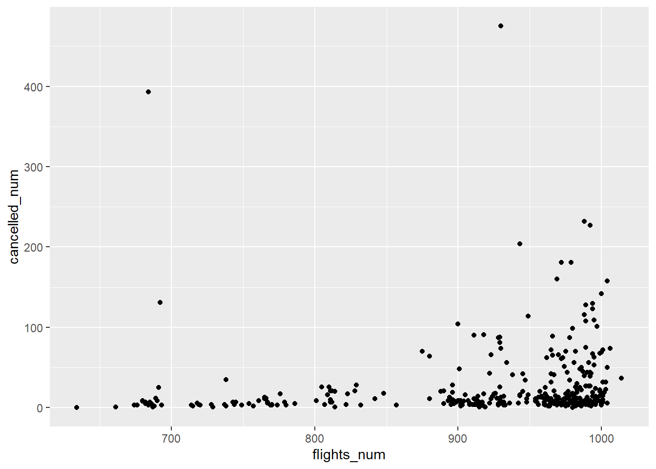
The second part of the question asks whether there is a relationship between the proportion of flights cancelled and the average departure delay. I implied this in my answer to the first part of the question, when I noted that increasing delays could result in increased cancellations. The question does not specify which delay, so I will show the relationship for both.
cancelled_and_delays <-
  flights %>%
  mutate(cancelled = (is.na(arr_delay) | is.na(dep_delay))) %>%
  group_by(year, month, day) %>%
  summarise(
    cancelled_prop = mean(cancelled),
    avg_dep_delay = mean(dep_delay, na.rm = TRUE),
    avg_arr_delay = mean(arr_delay, na.rm = TRUE)
  ) %>%
  ungroup()
## `summarise()` has grouped output by 'year', 'month'. You can override using the `.groups` argument.There is a strong increasing relationship between both average departure delay and
and average arrival delay and the proportion of cancelled flights.
ggplot(cancelled_and_delays) +
  geom_point(aes(x = avg_dep_delay, y = cancelled_prop))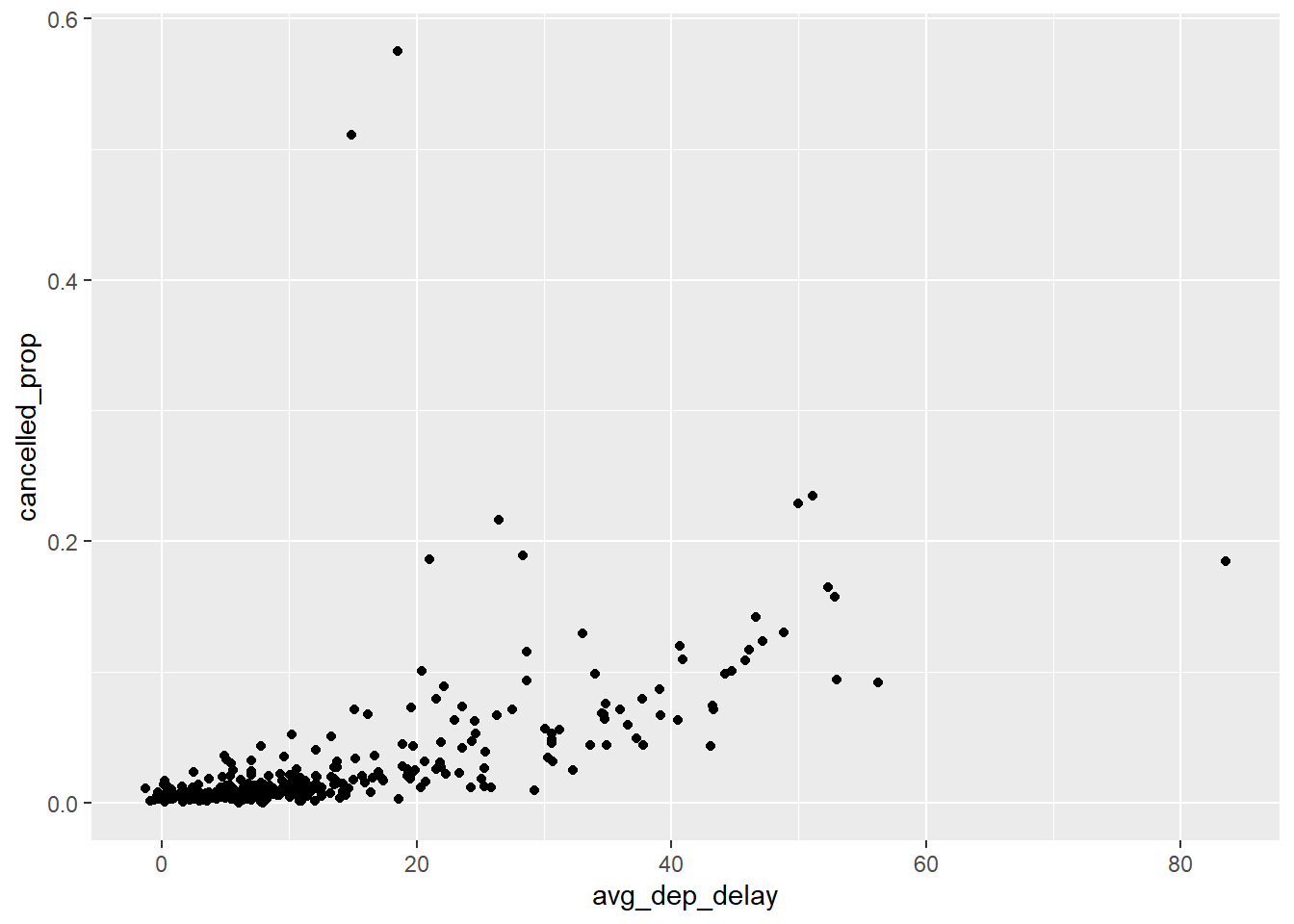
ggplot(cancelled_and_delays) +
  geom_point(aes(x = avg_arr_delay, y = cancelled_prop))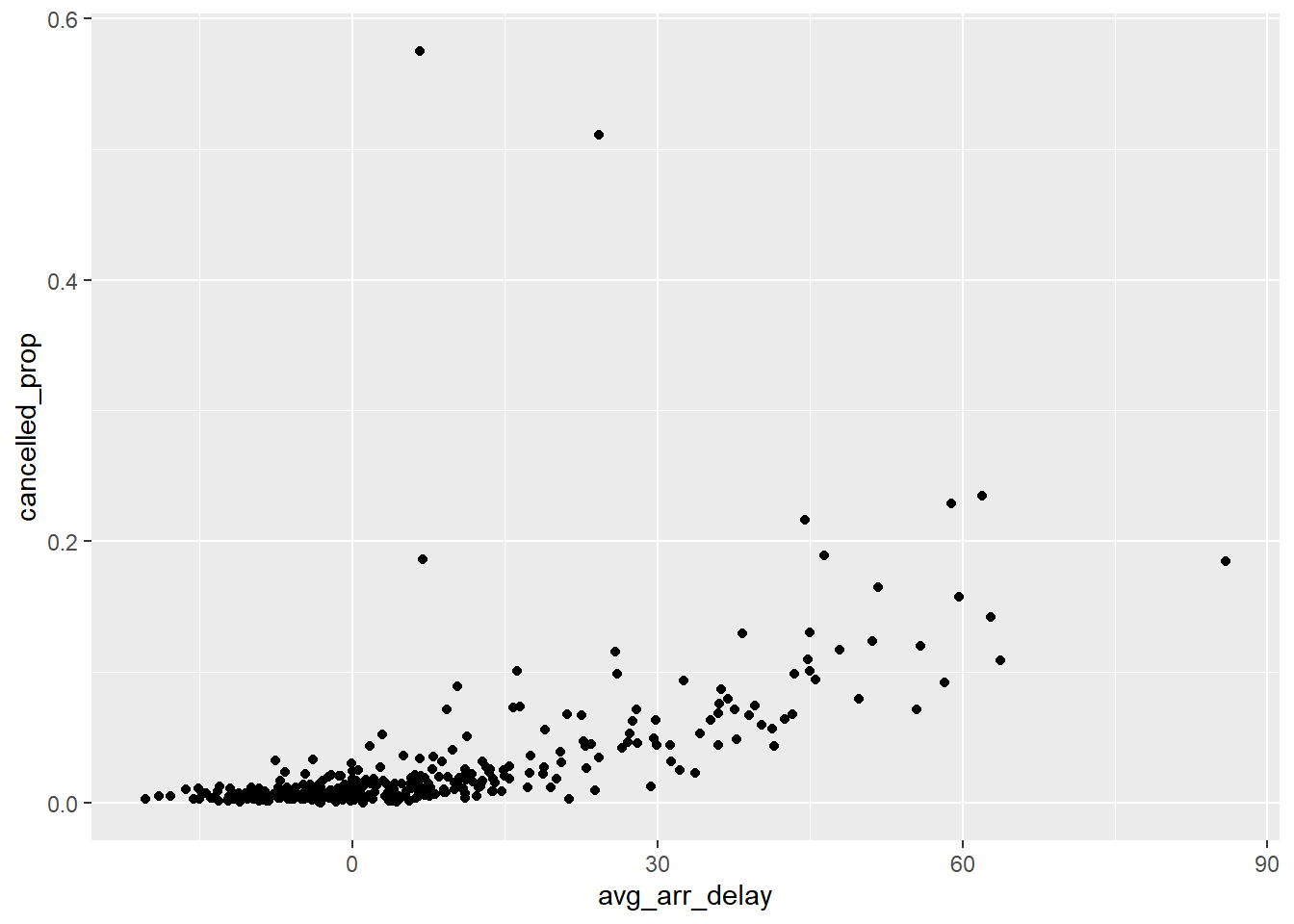
5.6.7.5
Which carrier has the worst delays? Challenge: can you disentangle the effects of bad airports vs. bad carriers? Why/why not? (Hint: think about
flights %>% group_by(carrier, dest) %>% summarise(n()))
flights %>%
  group_by(carrier) %>%
  summarise(arr_delay = mean(arr_delay, na.rm = TRUE)) %>%
  arrange(desc(arr_delay))
## # A tibble: 16 x 2
## carrier arr_delay
## <chr> <dbl>
## 1 F9 21.9
## 2 FL 20.1
## 3 EV 15.8
## 4 YV 15.6
## 5 OO 11.9
## 6 MQ 10.8
## 7 WN 9.65
## 8 B6 9.46
## 9 9E 7.38
## 10 UA 3.56
## 11 US 2.13
## 12 VX 1.76
## 13 DL 1.64
## 14 AA 0.364
## 15 HA -6.92
## 16 AS -9.93What airline corresponds to the "F9" carrier code?
filter(airlines, carrier == "F9")## # A tibble: 1 x 2
## carrier name
## <chr> <chr>
## 1 F9 Frontier Airlines Inc.You can get part of the way to disentangling the effects of airports versus bad carriers by comparing the average delay of each carrier to the average delay of flights within a route (flights from the same origin to the same destination). Comparing delays between carriers and within each route disentangles the effect of carriers and airports. A better analysis would compare the average delay of a carrier’s flights to the average delay of all other carrier’s flights within a route.
flights %>%
  filter(!is.na(arr_delay)) %>%
  # Total delay by carrier within each origin, dest
  group_by(origin, dest, carrier) %>%
  summarise(
    arr_delay = sum(arr_delay),
    flights = n()
  ) %>%
  # Total delay within each origin dest
  group_by(origin, dest) %>%
  mutate(
    arr_delay_total = sum(arr_delay),
    flights_total = sum(flights)
  ) %>%
  # average delay of each carrier - average delay of other carriers
  ungroup() %>%
  mutate(
    arr_delay_others = (arr_delay_total - arr_delay) /
      (flights_total - flights),
    arr_delay_mean = arr_delay / flights,
    arr_delay_diff = arr_delay_mean - arr_delay_others
  ) %>%
  # remove NaN values (when there is only one carrier)
  filter(is.finite(arr_delay_diff)) %>%
  # average over all airports it flies to
  group_by(carrier) %>%
  summarise(arr_delay_diff = mean(arr_delay_diff)) %>%
  arrange(desc(arr_delay_diff))
## `summarise()` has grouped output by 'origin', 'dest'. You can override using the `.groups` argument.## # A tibble: 15 x 2
## carrier arr_delay_diff
## <chr> <dbl>
## 1 OO 27.3
## 2 F9 17.3
## 3 EV 11.0
## 4 B6 6.41
## 5 FL 2.57
## 6 VX -0.202
## 7 AA -0.970
## 8 WN -1.27
## 9 UA -1.86
## 10 MQ -2.48
## 11 YV -2.81
## 12 9E -3.54
## 13 US -4.14
## 14 DL -10.2
## 15 AS -15.8There are more sophisticated ways to do this analysis, however comparing the delay of flights within each route goes a long ways toward disentangling airport and carrier effects. To see a more complete example of this analysis, see this FiveThirtyEight piece.
5.6.7.6
What does the sort argument to
count()do? When might you use it?
The sort argument to count() sorts the results in order of n.
You could use this anytime you would run count() followed by arrange().
For example, the following expression counts the number of flights to a destination and sorts the returned data from highest to lowest.
flights %>%
  count(dest, sort = TRUE)
## # A tibble: 105 x 2
## dest n
## <chr> <int>
## 1 ORD 17283
## 2 ATL 17215
## 3 LAX 16174
## 4 BOS 15508
## 5 MCO 14082
## 6 CLT 14064
## 7 SFO 13331
## 8 FLL 12055
## 9 MIA 11728
## 10 DCA 9705
## # ... with 95 more rowsExercise 5.7.1
Refer back to the lists of useful mutate and filtering functions. Describe how each operation changes when you combine it with grouping.
Summary functions (mean()), offset functions (lead(), lag()), ranking functions (min_rank(), row_number()), operate within each group when used with group_by() in
mutate() or filter().
Arithmetic operators (+, -), logical operators (<, ==), modular arithmetic operators (%%, %/%), logarithmic functions (log) are not affected by group_by.
Summary functions like mean(), median(), sum(), std() and others covered
in the section Useful Summary Functions
calculate their values within each group when used with mutate() or filter() and group_by().
tibble(x = 1:9,
       group = rep(c("a", "b", "c"), each = 3)) %>%
  mutate(x_mean = mean(x)) %>%
  group_by(group) %>%
  mutate(x_mean_2 = mean(x))
## # A tibble: 9 x 4
## # Groups: group [3]
## x group x_mean x_mean_2
## <int> <chr> <dbl> <dbl>
## 1 1 a 5 2
## 2 2 a 5 2
## 3 3 a 5 2
## 4 4 b 5 5
## 5 5 b 5 5
## 6 6 b 5 5
## 7 7 c 5 8
## 8 8 c 5 8
## 9 9 c 5 8Arithmetic operators +, -, *, /, ^ are not affected by group_by().
tibble(x = 1:9,
       group = rep(c("a", "b", "c"), each = 3)) %>%
  mutate(y = x + 2) %>%
  group_by(group) %>%
  mutate(z = x + 2)
## # A tibble: 9 x 4
## # Groups: group [3]
## x group y z
## <int> <chr> <dbl> <dbl>
## 1 1 a 3 3
## 2 2 a 4 4
## 3 3 a 5 5
## 4 4 b 6 6
## 5 5 b 7 7
## 6 6 b 8 8
## 7 7 c 9 9
## 8 8 c 10 10
## 9 9 c 11 11The modular arithmetic operators %/% and %% are not affected by group_by()
tibble(x = 1:9,
       group = rep(c("a", "b", "c"), each = 3)) %>%
  mutate(y = x %% 2) %>%
  group_by(group) %>%
  mutate(z = x %% 2)
## # A tibble: 9 x 4
## # Groups: group [3]
## x group y z
## <int> <chr> <dbl> <dbl>
## 1 1 a 1 1
## 2 2 a 0 0
## 3 3 a 1 1
## 4 4 b 0 0
## 5 5 b 1 1
## 6 6 b 0 0
## 7 7 c 1 1
## 8 8 c 0 0
## 9 9 c 1 1The logarithmic functions log(), log2(), and log10() are not affected by
group_by().
tibble(x = 1:9,
       group = rep(c("a", "b", "c"), each = 3)) %>%
  mutate(y = log(x)) %>%
  group_by(group) %>%
  mutate(z = log(x))
## # A tibble: 9 x 4
## # Groups: group [3]
## x group y z
## <int> <chr> <dbl> <dbl>
## 1 1 a 0 0
## 2 2 a 0.693 0.693
## 3 3 a 1.10 1.10
## 4 4 b 1.39 1.39
## 5 5 b 1.61 1.61
## 6 6 b 1.79 1.79
## 7 7 c 1.95 1.95
## 8 8 c 2.08 2.08
## 9 9 c 2.20 2.20The offset functions lead() and lag() respect the groupings in group_by().
The functions lag() and lead() will only return values within each group.
tibble(x = 1:9,
       group = rep(c("a", "b", "c"), each = 3)) %>%
  group_by(group) %>%
  mutate(lag_x = lag(x),
         lead_x = lead(x))
## # A tibble: 9 x 4
## # Groups: group [3]
## x group lag_x lead_x
## <int> <chr> <int> <int>
## 1 1 a NA 2
## 2 2 a 1 3
## 3 3 a 2 NA
## 4 4 b NA 5
## 5 5 b 4 6
## 6 6 b 5 NA
## 7 7 c NA 8
## 8 8 c 7 9
## 9 9 c 8 NAThe cumulative and rolling aggregate functions cumsum(), cumprod(), cummin(), cummax(), and cummean() calculate values within each group.
tibble(x = 1:9,
       group = rep(c("a", "b", "c"), each = 3)) %>%
  mutate(x_cumsum = cumsum(x)) %>%
  group_by(group) %>%
  mutate(x_cumsum_2 = cumsum(x))
## # A tibble: 9 x 4
## # Groups: group [3]
## x group x_cumsum x_cumsum_2
## <int> <chr> <int> <int>
## 1 1 a 1 1
## 2 2 a 3 3
## 3 3 a 6 6
## 4 4 b 10 4
## 5 5 b 15 9
## 6 6 b 21 15
## 7 7 c 28 7
## 8 8 c 36 15
## 9 9 c 45 24Logical comparisons, <, <=, >, >=, !=, and == are not affected by group_by().
tibble(x = 1:9,
       y = 9:1,
       group = rep(c("a", "b", "c"), each = 3)) %>%
  mutate(x_lte_y = x <= y) %>%
  group_by(group) %>%
  mutate(x_lte_y_2 = x <= y)
## # A tibble: 9 x 5
## # Groups: group [3]
## x y group x_lte_y x_lte_y_2
## <int> <int> <chr> <lgl> <lgl>
## 1 1 9 a TRUE TRUE
## 2 2 8 a TRUE TRUE
## 3 3 7 a TRUE TRUE
## 4 4 6 b TRUE TRUE
## 5 5 5 b TRUE TRUE
## 6 6 4 b FALSE FALSE
## 7 7 3 c FALSE FALSE
## 8 8 2 c FALSE FALSE
## 9 9 1 c FALSE FALSERanking functions like min_rank() work within each group when used with group_by().
tibble(x = 1:9,
       group = rep(c("a", "b", "c"), each = 3)) %>%
  mutate(rnk = min_rank(x)) %>%
  group_by(group) %>%
  mutate(rnk2 = min_rank(x))
## # A tibble: 9 x 4
## # Groups: group [3]
## x group rnk rnk2
## <int> <chr> <int> <int>
## 1 1 a 1 1
## 2 2 a 2 2
## 3 3 a 3 3
## 4 4 b 4 1
## 5 5 b 5 2
## 6 6 b 6 3
## 7 7 c 7 1
## 8 8 c 8 2
## 9 9 c 9 3Though not asked in the question, note that arrange() ignores groups when sorting values.
tibble(x = runif(9),
       group = rep(c("a", "b", "c"), each = 3)) %>%
  group_by(group) %>%
  arrange(x)
## # A tibble: 9 x 2
## # Groups: group [3]
## x group
## <dbl> <chr>
## 1 0.0941 a
## 2 0.170 b
## 3 0.606 a
## 4 0.729 c
## 5 0.744 b
## 6 0.874 b
## 7 0.897 c
## 8 0.932 a
## 9 0.956 cHowever, the order of values from arrange() can interact with groups when
used with functions that rely on the ordering of elements, such as lead(), lag(),
or cumsum().
tibble(group = rep(c("a", "b", "c"), each = 3),
       x = runif(9)) %>%
  group_by(group) %>%
  arrange(x) %>%
  mutate(lag_x = lag(x))
## # A tibble: 9 x 3
## # Groups: group [3]
## group x lag_x
## <chr> <dbl> <dbl>
## 1 a 0.00549 NA
## 2 c 0.109 NA
## 3 a 0.152 0.00549
## 4 a 0.351 0.152
## 5 c 0.552 0.109
## 6 b 0.576 NA
## 7 b 0.768 0.576
## 8 c 0.810 0.552
## 9 b 0.885 0.7685.7.1.2
Which plane (
tailnum) has the worst on-time record?
The question does not define a way to measure on-time record, so I will consider two metrics:
- proportion of flights not delayed or cancelled, and
- mean arrival delay.
The first metric is the proportion of not-cancelled and on-time flights. I use the presence of an arrival time as an indicator that a flight was not cancelled. However, there are many planes that have never flown an on-time flight. Additionally, many of the planes that have the lowest proportion of on-time flights have only flown a small number of flights.
flights %>%
  filter(!is.na(tailnum)) %>%
  mutate(on_time = !is.na(arr_time) & (arr_delay <= 0)) %>%
  group_by(tailnum) %>%
  summarise(on_time = mean(on_time), n = n()) %>%
  filter(min_rank(on_time) == 1)
## # A tibble: 110 x 3
## tailnum on_time n
## <chr> <dbl> <int>
## 1 N121DE 0 2
## 2 N136DL 0 1
## 3 N143DA 0 1
## 4 N17627 0 2
## 5 N240AT 0 5
## 6 N26906 0 1
## 7 N295AT 0 4
## 8 N302AS 0 1
## 9 N303AS 0 1
## 10 N32626 0 1
## # ... with 100 more rowsSo, I will remove planes that flew at least 20 flights. The choice of 20 was chosen because it round number near the first quartile of the number of flights by plane.12
quantile(count(flights, tailnum)$n)## 0% 25% 50% 75% 100%
## 1 23 54 110 2512The plane with the worst on time record that flew at least 20 flights is:
flights %>%
  filter(!is.na(tailnum), is.na(arr_time) | !is.na(arr_delay)) %>%
  mutate(on_time = !is.na(arr_time) & (arr_delay <= 0)) %>%
  group_by(tailnum) %>%
  summarise(on_time = mean(on_time), n = n()) %>%
  filter(n >= 20) %>%
  filter(min_rank(on_time) == 1)
## # A tibble: 1 x 3
## tailnum on_time n
## <chr> <dbl> <int>
## 1 N988AT 0.189 37There are cases where arr_delay is missing but arr_time is not missing.
I have not debugged the cause of this bad data, so these rows are dropped for
the purposes of this exercise.
The second metric is the mean minutes delayed. As with the previous metric, I will only consider planes which flew least 20 flights. A different plane has the worst on-time record when measured as average minutes delayed.
flights %>%
  filter(!is.na(arr_delay)) %>%
  group_by(tailnum) %>%
  summarise(arr_delay = mean(arr_delay), n = n()) %>%
  filter(n >= 20) %>%
  filter(min_rank(desc(arr_delay)) == 1)
## # A tibble: 1 x 3
## tailnum arr_delay n
## <chr> <dbl> <int>
## 1 N203FR 59.1 415.7.1.3
What time of day should you fly if you want to avoid delays as much as possible?
Let’s group by the hour of the flight. The earlier the flight is scheduled, the lower its expected delay. This is intuitive as delays will affect later flights. Morning flights have fewer (if any) previous flights that can delay them.
flights %>%
  group_by(hour) %>%
  summarise(arr_delay = mean(arr_delay, na.rm = TRUE)) %>%
  arrange(arr_delay)
## # A tibble: 20 x 2
## hour arr_delay
## <dbl> <dbl>
## 1 7 -5.30
## 2 5 -4.80
## 3 6 -3.38
## 4 9 -1.45
## 5 8 -1.11
## 6 10 0.954
## 7 11 1.48
## 8 12 3.49
## 9 13 6.54
## 10 14 9.20
## 11 23 11.8
## 12 15 12.3
## 13 16 12.6
## 14 18 14.8
## 15 22 16.0
## 16 17 16.0
## 17 19 16.7
## 18 20 16.7
## 19 21 18.4
## 20 1 NaN5.7.1.4
For each destination, compute the total minutes of delay. For each flight, compute the proportion of the total delay for its destination.
The key to answering this question is to only include delayed flights when calculating the total delay and proportion of delay.
flights %>%
  filter(arr_delay > 0) %>%
  group_by(dest) %>%
  mutate(
    arr_delay_total = sum(arr_delay),
    arr_delay_prop = arr_delay / arr_delay_total
  ) %>%
  select(dest, month, day, dep_time, carrier, flight,
         arr_delay, arr_delay_prop) %>%
  arrange(dest, desc(arr_delay_prop))
## # A tibble: 133,004 x 8
## # Groups: dest [103]
## dest month day dep_time carrier flight arr_delay arr_delay_prop
## <chr> <int> <int> <int> <chr> <int> <dbl> <dbl>
## 1 ABQ 7 22 2145 B6 1505 153 0.0341
## 2 ABQ 12 14 2223 B6 65 149 0.0332
## 3 ABQ 10 15 2146 B6 65 138 0.0308
## 4 ABQ 7 23 2206 B6 1505 137 0.0305
## 5 ABQ 12 17 2220 B6 65 136 0.0303
## 6 ABQ 7 10 2025 B6 1505 126 0.0281
## 7 ABQ 7 30 2212 B6 1505 118 0.0263
## 8 ABQ 7 28 2038 B6 1505 117 0.0261
## 9 ABQ 12 8 2049 B6 65 114 0.0254
## 10 ABQ 9 2 2212 B6 1505 109 0.0243
## # ... with 132,994 more rowsThere is some ambiguity in the meaning of the term flights in the question.
The first example defined a flight as a row in the flights table, which is a trip by an aircraft from an airport at a particular date and time.
However, flight could also refer to the flight number, which is the code a carrier uses for an airline service of a route.
For example, AA1 is the flight number of the 09:00 American Airlines flight between JFK and LAX.
The flight number is contained in the flights$flight column, though what is called a “flight” is a combination of the flights$carrier and flights$flight columns.
flights %>%
  filter(arr_delay > 0) %>%
  group_by(dest, origin, carrier, flight) %>%
  summarise(arr_delay = sum(arr_delay)) %>%
  group_by(dest) %>%
  mutate(
    arr_delay_prop = arr_delay / sum(arr_delay)
  ) %>%
  arrange(dest, desc(arr_delay_prop)) %>%
  select(carrier, flight, origin, dest, arr_delay_prop)
## `summarise()` has grouped output by 'dest', 'origin', 'carrier'. You can override using the `.groups` argument.## # A tibble: 8,834 x 5
## # Groups: dest [103]
## carrier flight origin dest arr_delay_prop
## <chr> <int> <chr> <chr> <dbl>
## 1 B6 1505 JFK ABQ 0.567
## 2 B6 65 JFK ABQ 0.433
## 3 B6 1191 JFK ACK 0.475
## 4 B6 1491 JFK ACK 0.414
## 5 B6 1291 JFK ACK 0.0898
## 6 B6 1195 JFK ACK 0.0208
## 7 EV 4309 EWR ALB 0.174
## 8 EV 4271 EWR ALB 0.137
## 9 EV 4117 EWR ALB 0.0951
## 10 EV 4088 EWR ALB 0.0865
## # ... with 8,824 more rows5.7.1.5
Delays are typically temporally correlated: even once the problem that caused the initial delay has been resolved, later >flights are delayed to allow earlier flights to leave. Using
lag()explore how the delay of a flight is related to the >delay of the immediately preceding flight.
This calculates the departure delay of the preceding flight from the same airport.
lagged_delays <- flights %>%
  arrange(origin, month, day, dep_time) %>%
  group_by(origin) %>%
  mutate(dep_delay_lag = lag(dep_delay)) %>%
  filter(!is.na(dep_delay), !is.na(dep_delay_lag))
This plots the relationship between the mean delay of a flight for all values of the previous flight. For delays less than two hours, the relationship between the delay of the preceding flight and the current flight is nearly a line. After that the relationship becomes more variable, as long-delayed flights are interspersed with flights leaving on-time. After about 8-hours, a delayed flight is likely to be followed by a flight leaving on time.
lagged_delays %>%
  group_by(dep_delay_lag) %>%
  summarise(dep_delay_mean = mean(dep_delay)) %>%
  ggplot(aes(y = dep_delay_mean, x = dep_delay_lag)) +
  geom_point() +
  scale_x_continuous(breaks = seq(0, 1500, by = 120)) +
  labs(y = "Departure Delay", x = "Previous Departure Delay")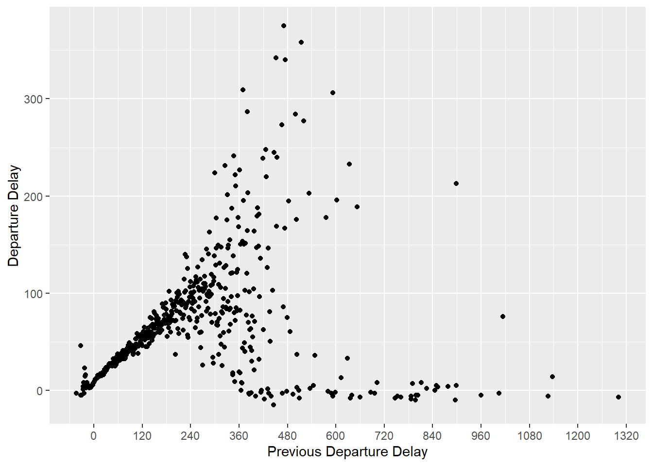
The overall relationship looks similar in all three origin airports.
lagged_delays %>%
  group_by(origin, dep_delay_lag) %>%
  summarise(dep_delay_mean = mean(dep_delay)) %>%
  ggplot(aes(y = dep_delay_mean, x = dep_delay_lag)) +
  geom_point() +
  facet_wrap(~ origin, ncol=1) +
  labs(y = "Departure Delay", x = "Previous Departure Delay")
## `summarise()` has grouped output by 'origin'. You can override using the `.groups` argument.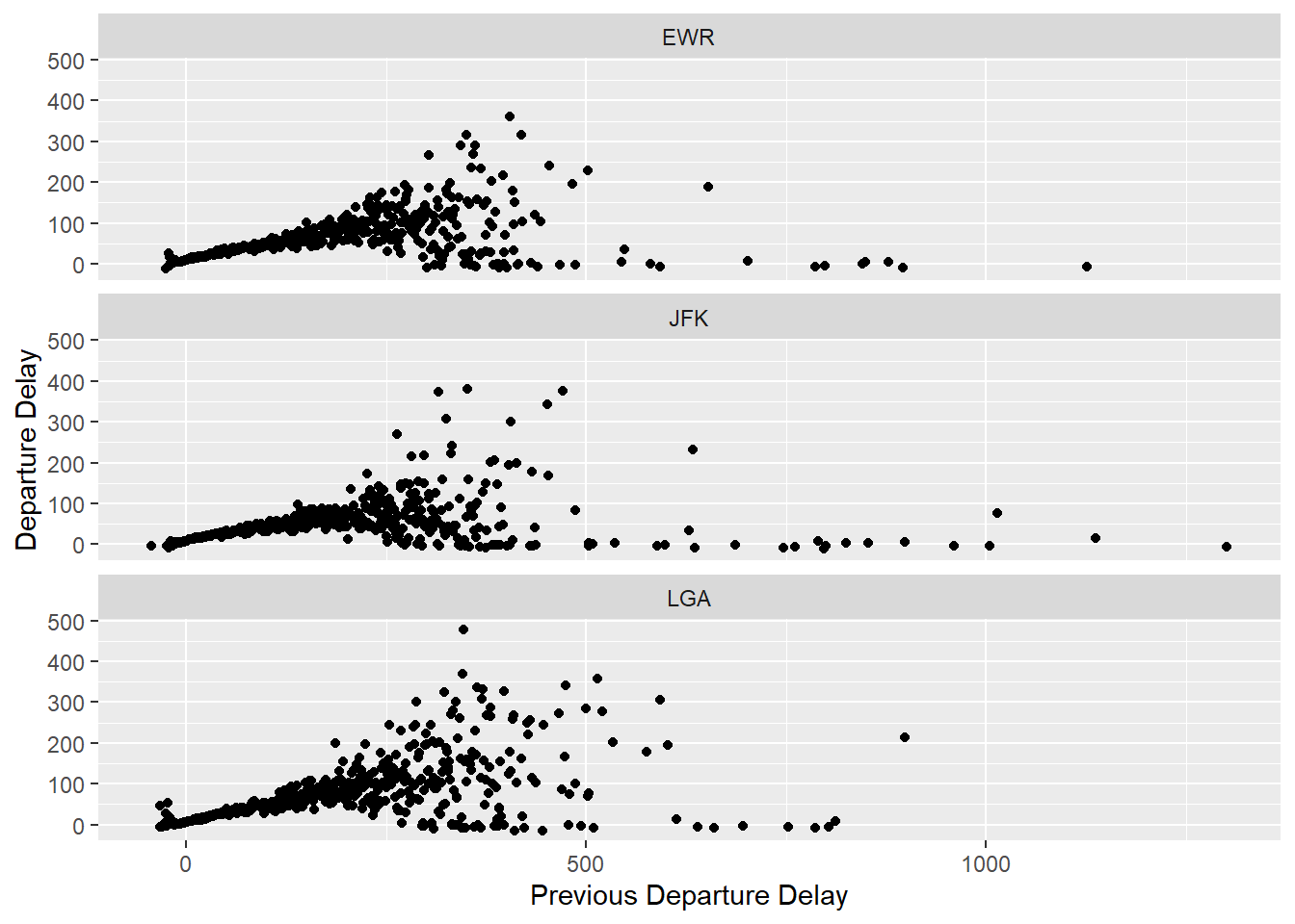
5.7.1.6
Look at each destination. Can you find flights that are suspiciously fast? (i.e. flights that represent a potential data entry error). Compute the air time of a flight relative to the shortest flight to that destination. Which flights were most delayed in the air?
When calculating this answer we should only compare flights within the same (origin, destination) pair.
To find unusual observations, we need to first put them on the same scale. I will standardize values by subtracting the mean from each and then dividing each by the standard deviation. \[ \mathsf{standardized}(x) = \frac{x - \mathsf{mean}(x)}{\mathsf{sd}(x)} . \] A standardized variable is often called a \(z\)-score. The units of the standardized variable are standard deviations from the mean. This will put the flight times from different routes on the same scale. The larger the magnitude of the standardized variable for an observation, the more unusual the observation is. Flights with negative values of the standardized variable are faster than the mean flight for that route, while those with positive values are slower than the mean flight for that route.
standardized_flights <- flights %>%
  filter(!is.na(air_time)) %>%
  group_by(dest, origin) %>%
  mutate(
    air_time_mean = mean(air_time),
    air_time_sd = sd(air_time),
    n = n()
  ) %>%
  ungroup() %>%
  mutate(air_time_standard = (air_time - air_time_mean) / (air_time_sd + 1))
I add 1 to the denominator and numerator to avoid dividing by zero.
Note that the ungroup() here is not necessary. However, I will be using
this data frame later. Through experience, I have found that I have fewer bugs
when I keep a data frame grouped for only those verbs that need it.
If I did not ungroup() this data frame, the arrange() used later would
not work as expected. It is better to err on the side of using ungroup()
when unnecessary.
The distribution of the standardized air flights has long right tail.
ggplot(standardized_flights, aes(x = air_time_standard)) +
  geom_density()
## Warning: Removed 4 rows containing non-finite values (stat_density).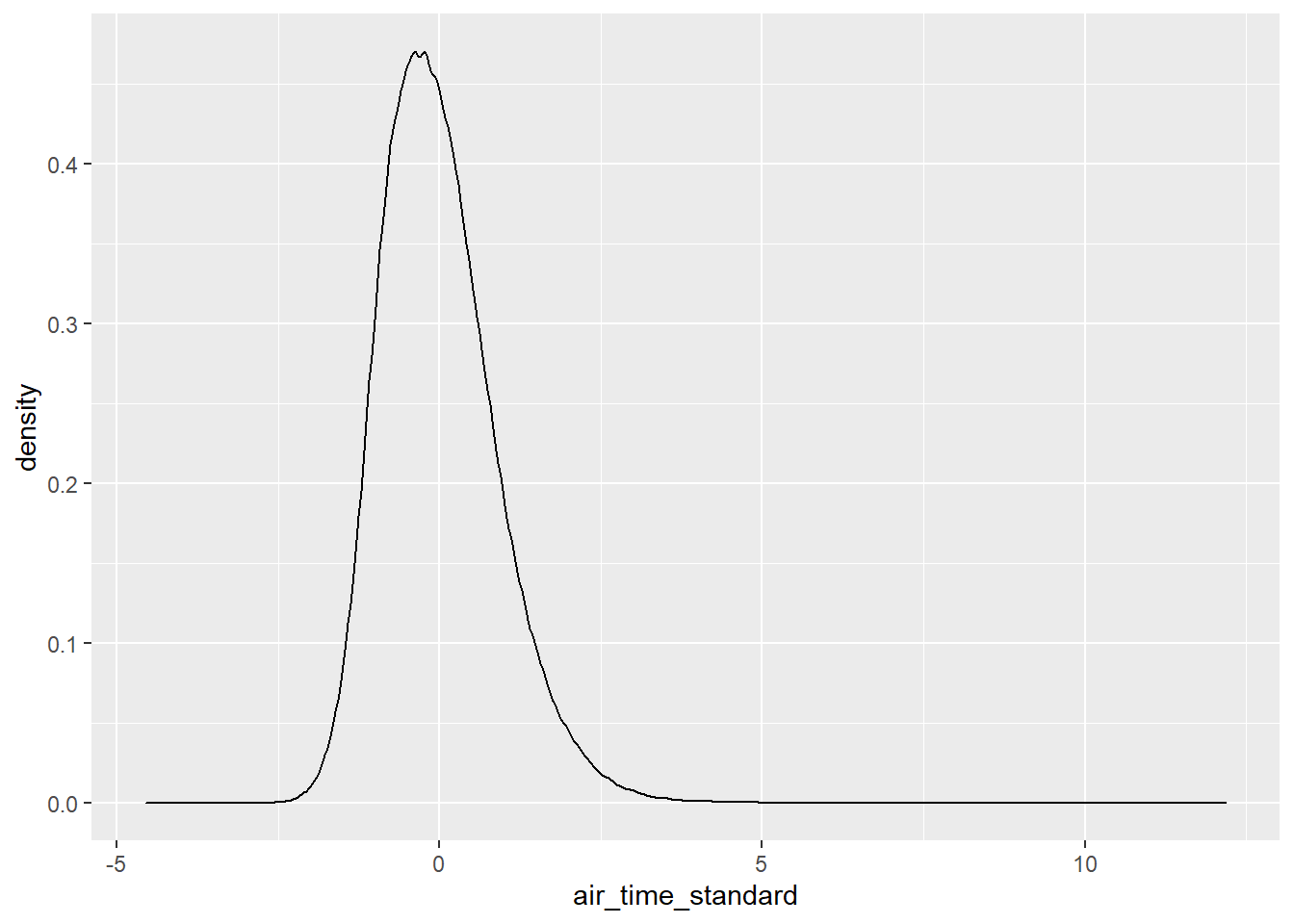
Unusually fast flights are those flights with the smallest standardized values.
standardized_flights %>%
  arrange(air_time_standard) %>%
  select(
    carrier, flight, origin, dest, month, day,
    air_time, air_time_mean, air_time_standard
  ) %>%
  head(10) %>%
  print(width = Inf)
## # A tibble: 10 x 9
## carrier flight origin dest month day air_time air_time_mean
## <chr> <int> <chr> <chr> <int> <int> <dbl> <dbl>
## 1 DL 1499 LGA ATL 5 25 65 114.
## 2 EV 4667 EWR MSP 7 2 93 151.
## 3 EV 4292 EWR GSP 5 13 55 93.2
## 4 EV 3805 EWR BNA 3 23 70 115.
## 5 EV 4687 EWR CVG 9 29 62 96.1
## 6 B6 2002 JFK BUF 11 10 38 57.1
## 7 DL 1902 LGA PBI 1 12 105 146.
## 8 DL 161 JFK SEA 7 3 275 329.
## 9 EV 5486 LGA PIT 4 28 40 57.7
## 10 B6 30 JFK ROC 3 25 35 51.9
## air_time_standard
## <dbl>
## 1 -4.56
## 2 -4.46
## 3 -4.20
## 4 -3.73
## 5 -3.60
## 6 -3.38
## 7 -3.34
## 8 -3.34
## 9 -3.15
## 10 -3.10I used width = Inf to ensure that all columns will be printed.
The fastest flight is DL1499 from LGA to ATL which departed on 2013-05-25 at 17:09. It has an air time of 65 minutes, compared to an average flight time of 114 minutes for its route. This is 4.6 standard deviations below the average flight on its route.
It is important to note that this does not necessarily imply that there was a data entry error. We should check these flights to see whether there was some reason for the difference. It may be that we are missing some piece of information that explains these unusual times.
A potential issue with the way that we standardized the flights is that the mean and standard deviation used to calculate are sensitive to outliers and outliers is what we are looking for. Instead of standardizing variables with the mean and variance, we could use the median as a measure of central tendency and the interquartile range (IQR) as a measure of spread. The median and IQR are more resistant to outliers than the mean and standard deviation. The following method uses the median and inter-quartile range, which are less sensitive to outliers.
standardized_flights2 <- flights %>%
  filter(!is.na(air_time)) %>%
  group_by(dest, origin) %>%
  mutate(
    air_time_median = median(air_time),
    air_time_iqr = IQR(air_time),
    n = n(),
    air_time_standard = (air_time - air_time_median) / air_time_iqr)
The distribution of the standardized air flights using this new definition also has long right tail of slow flights.
ggplot(standardized_flights2, aes(x = air_time_standard)) +
  geom_density()
## Warning: Removed 4 rows containing non-finite values (stat_density).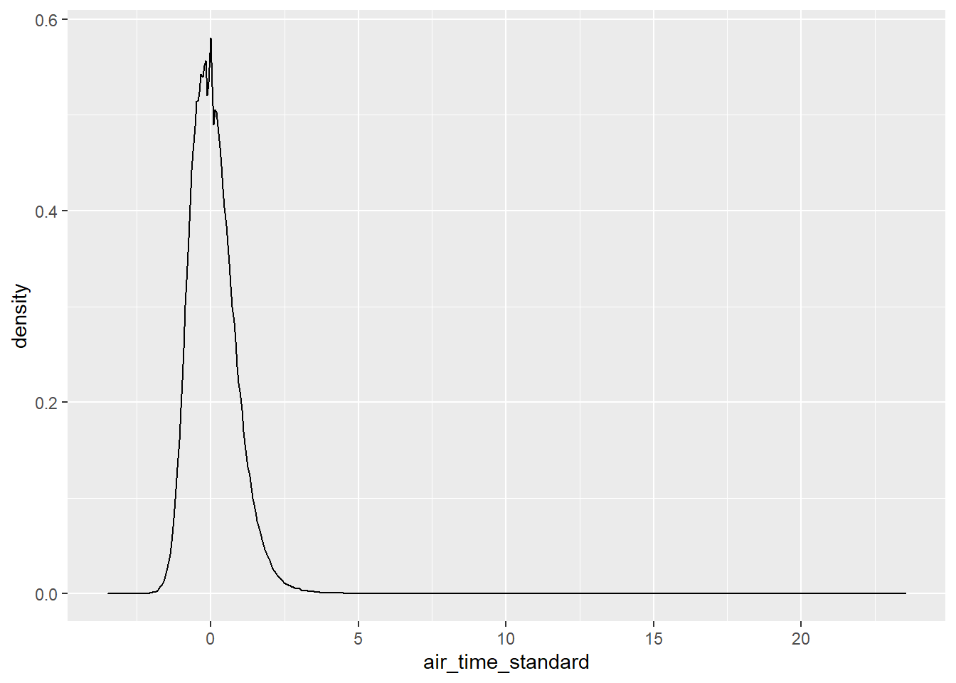
Unusually fast flights are those flights with the smallest standardized values.
standardized_flights2 %>%
  arrange(air_time_standard) %>%
  select(
    carrier, flight, origin, dest, month, day, air_time,
    air_time_median, air_time_standard
  ) %>%
  head(10) %>%
  print(width = Inf)
## # A tibble: 10 x 9
## # Groups: dest, origin [10]
## carrier flight origin dest month day air_time air_time_median
## <chr> <int> <chr> <chr> <int> <int> <dbl> <dbl>
## 1 EV 4667 EWR MSP 7 2 93 149
## 2 DL 1499 LGA ATL 5 25 65 112
## 3 US 2132 LGA BOS 3 2 21 37
## 4 B6 30 JFK ROC 3 25 35 51
## 5 B6 2002 JFK BUF 11 10 38 57
## 6 EV 4292 EWR GSP 5 13 55 92
## 7 EV 4249 EWR SYR 3 15 30 39
## 8 EV 4580 EWR BTV 6 29 34 46
## 9 EV 3830 EWR RIC 7 2 35 53
## 10 EV 4687 EWR CVG 9 29 62 95
## air_time_standard
## <dbl>
## 1 -3.5
## 2 -3.36
## 3 -3.2
## 4 -3.2
## 5 -3.17
## 6 -3.08
## 7 -3
## 8 -3
## 9 -3
## 10 -3All of these answers have relied only on using a distribution of comparable observations to find unusual observations.
In this case, the comparable observations were flights from the same origin to the same destination.
Apart from our knowledge that flights from the same origin to the same destination should have similar air times, we have not used any other domain-specific knowledge.
But we know much more about this problem.
The most obvious piece of knowledge we have is that we know that flights cannot travel back in time, so there should never be a flight with a negative airtime.
But we also know that aircraft have maximum speeds.
While different aircraft have different cruising speeds, commercial airliners
typically cruise at air speeds around 547–575 mph.
Calculating the ground speed of aircraft is complicated by the way in which winds, especially the influence of wind, especially jet streams, on the ground-speed of flights.
A strong tailwind can increase ground-speed of the aircraft by 200 mph.
Apart from the retired Concorde.
For example, in 2018, a transatlantic flight
traveled at 770 mph due to a strong jet stream tailwind.
This means that any flight traveling at speeds greater than 800 mph is implausible,
and it may be worth checking flights traveling at greater than 600 or 700 mph.
Ground speed could also be used to identify aircraft flying implausibly slow.
Joining flights data with the air craft type in the planes table and getting
information about typical or top speeds of those aircraft could provide a more
detailed way to identify implausibly fast or slow flights.
Additional data on high altitude wind speeds at the time of the flight would further help.
Knowing the substance of the data analysis at hand is one of the most important tools of a data scientist. The tools of statistics are a complement, not a substitute, for that knowledge.
With that in mind, Let’s plot the distribution of the ground speed of flights. The modal flight in this data has a ground speed of between 400 and 500 mph. The distribution of ground speeds has a large left tail of slower flights below 400 mph constituting the majority. There are very few flights with a ground speed over 500 mph.
flights %>%
  mutate(mph = distance / (air_time / 60)) %>%
  ggplot(aes(x = mph)) +
  geom_histogram(binwidth = 10)
## Warning: Removed 9430 rows containing non-finite values (stat_bin).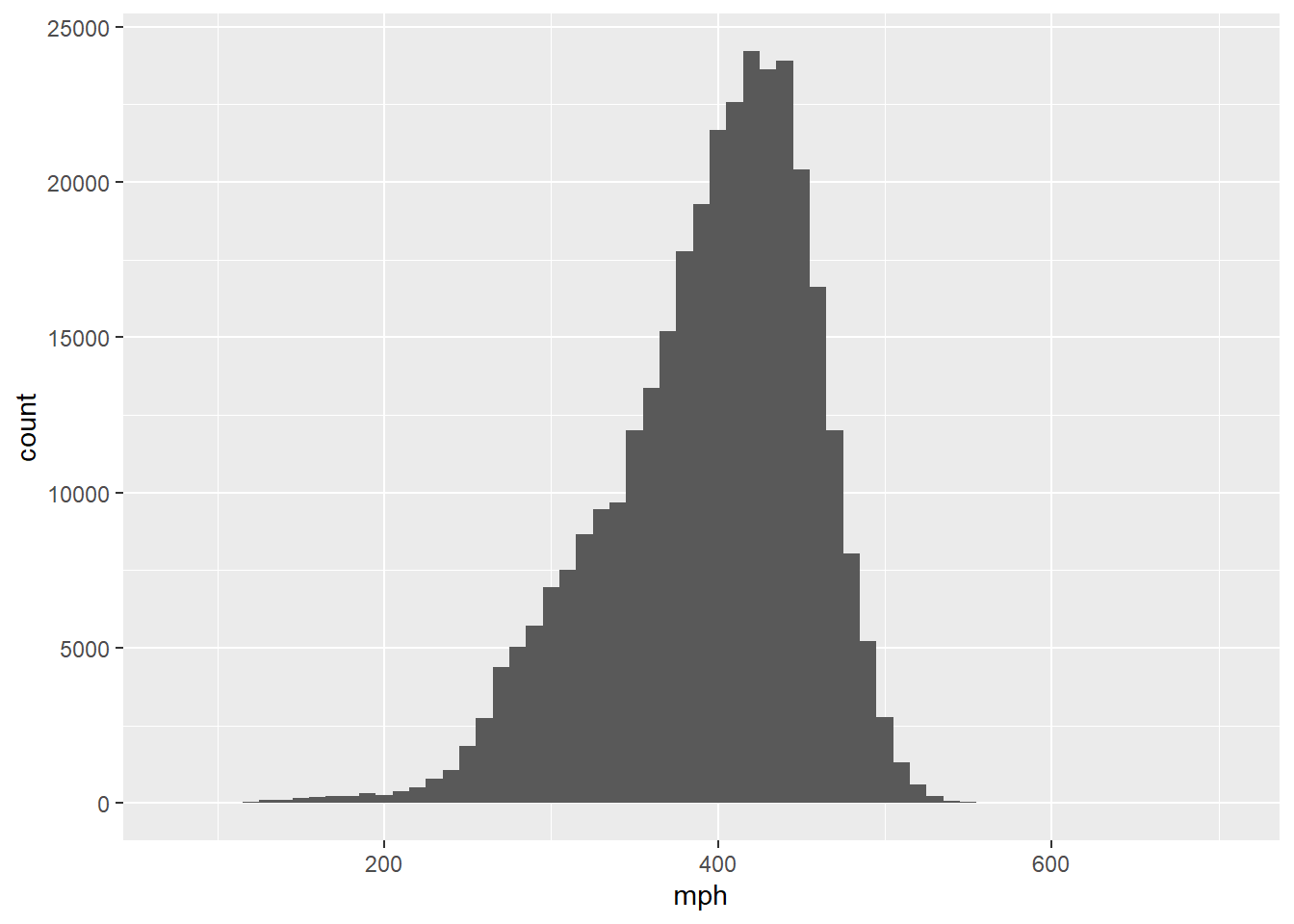
The fastest flight is the same one identified as the largest outlier earlier. Its ground speed was 703 mph. This is fast for a commercial jet, but not impossible.
flights %>%
  mutate(mph = distance / (air_time / 60)) %>%
  arrange(desc(mph)) %>%
  select(mph, flight, carrier, flight, month, day, dep_time) %>%
  head(5)
## # A tibble: 5 x 6
## mph flight carrier month day dep_time
## <dbl> <int> <chr> <int> <int> <int>
## 1 703. 1499 DL 5 25 1709
## 2 650. 4667 EV 7 2 1558
## 3 648 4292 EV 5 13 2040
## 4 641. 3805 EV 3 23 1914
## 5 591. 1902 DL 1 12 1559One explanation for unusually fast flights is that they are “making up time” in the air by flying faster. Commercial aircraft do not fly at their top speed since the airlines are also concerned about fuel consumption. But, if a flight is delayed on the ground, it may fly faster than usual in order to avoid a late arrival. So, I would expect that some of the unusually fast flights were delayed on departure.
flights %>%
  mutate(mph = distance / (air_time / 60)) %>%
  arrange(desc(mph)) %>%
  select(
    origin, dest, mph, year, month, day, dep_time, flight, carrier,
    dep_delay, arr_delay
  )
## # A tibble: 336,776 x 11
## origin dest mph year month day dep_time flight carrier dep_delay
## <chr> <chr> <dbl> <int> <int> <int> <int> <int> <chr> <dbl>
## 1 LGA ATL 703. 2013 5 25 1709 1499 DL 9
## 2 EWR MSP 650. 2013 7 2 1558 4667 EV 45
## 3 EWR GSP 648 2013 5 13 2040 4292 EV 15
## 4 EWR BNA 641. 2013 3 23 1914 3805 EV 4
## 5 LGA PBI 591. 2013 1 12 1559 1902 DL -1
## 6 JFK SJU 564 2013 11 17 650 315 DL -5
## 7 JFK SJU 557. 2013 2 21 2355 707 B6 -3
## 8 JFK STT 556. 2013 11 17 759 936 AA -1
## 9 JFK SJU 554. 2013 11 16 2003 347 DL 38
## 10 JFK SJU 554. 2013 11 16 2349 1503 B6 -10
## # ... with 336,766 more rows, and 1 more variable: arr_delay <dbl>head(5)## [1] 5Five of the top ten flights had departure delays, and three of those were able to make up that time in the air and arrive ahead of schedule.
Overall, there were a few flights that seemed unusually fast, but they all fall into the realm of plausibility and likely are not data entry problems. [Ed. Please correct me if I am missing something]
The second part of the question asks us to compare flights to the fastest flight
on a route to find the flights most delayed in the air. I will calculate the
amount a flight is delayed in air in two ways.
The first is the absolute delay, defined as the number of minutes longer than the fastest flight on that route,air_time - min(air_time).
The second is the relative delay, which is the percentage increase in air time relative to the time of the fastest flight
along that route, (air_time - min(air_time)) / min(air_time) * 100.
air_time_delayed <-
  flights %>%
  group_by(origin, dest) %>%
  mutate(
    air_time_min = min(air_time, na.rm = TRUE),
    air_time_delay = air_time - air_time_min,
    air_time_delay_pct = air_time_delay / air_time_min * 100
  )
## Warning in min(air_time, na.rm = TRUE): no non-missing arguments to min;
## returning InfThe most delayed flight in air in minutes was DL841 from JFK to SFO which departed on 2013-07-28 at 17:27. It took 189 minutes longer than the flight with the shortest air time on its route.
air_time_delayed %>%
  arrange(desc(air_time_delay)) %>%
  select(
    air_time_delay, carrier, flight,
    origin, dest, year, month, day, dep_time,
    air_time, air_time_min
  ) %>%
  head() %>%
  print(width = Inf)
## # A tibble: 6 x 11
## # Groups: origin, dest [5]
## air_time_delay carrier flight origin dest year month day dep_time air_time
## <dbl> <chr> <int> <chr> <chr> <int> <int> <int> <int> <dbl>
## 1 189 DL 841 JFK SFO 2013 7 28 1727 490
## 2 165 DL 426 JFK LAX 2013 11 22 1812 440
## 3 163 AA 575 JFK EGE 2013 1 28 1806 382
## 4 147 DL 17 JFK LAX 2013 7 10 1814 422
## 5 145 UA 745 LGA DEN 2013 9 10 1513 331
## 6 143 UA 587 EWR LAS 2013 11 22 2142 399
## air_time_min
## <dbl>
## 1 301
## 2 275
## 3 219
## 4 275
## 5 186
## 6 256The most delayed flight in air as a percentage of the fastest flight along that route was US2136 from LGA to BOS departing on 2013-06-17 at 16:52. It took 410% longer than the flight with the shortest air time on its route.
air_time_delayed %>%
  arrange(desc(air_time_delay)) %>%
  select(
    air_time_delay_pct, carrier, flight,
    origin, dest, year, month, day, dep_time,
    air_time, air_time_min
  ) %>%
  head() %>%
  print(width = Inf)
## # A tibble: 6 x 11
## # Groups: origin, dest [5]
## air_time_delay_pct carrier flight origin dest year month day dep_time
## <dbl> <chr> <int> <chr> <chr> <int> <int> <int> <int>
## 1 62.8 DL 841 JFK SFO 2013 7 28 1727
## 2 60 DL 426 JFK LAX 2013 11 22 1812
## 3 74.4 AA 575 JFK EGE 2013 1 28 1806
## 4 53.5 DL 17 JFK LAX 2013 7 10 1814
## 5 78.0 UA 745 LGA DEN 2013 9 10 1513
## 6 55.9 UA 587 EWR LAS 2013 11 22 2142
## air_time air_time_min
## <dbl> <dbl>
## 1 490 301
## 2 440 275
## 3 382 219
## 4 422 275
## 5 331 186
## 6 399 2565.7.1.7
Find all destinations that are flown by at least two carriers. Use that information to rank the carriers.
To restate this question, we are asked to rank airlines by the number of destinations that they fly to, considering only those airports that are flown to by two or more airlines. There are two steps to calculating this ranking. First, find all airports serviced by two or more carriers. Then, rank carriers by the number of those destinations that they service.
flights %>%
   # find all airports with > 1 carrier
   group_by(dest) %>%
   mutate(n_carriers = n_distinct(carrier)) %>%
   filter(n_carriers > 1) %>%
   # rank carriers by numer of destinations
   group_by(carrier) %>%
   summarize(n_dest = n_distinct(dest)) %>%
   arrange(desc(n_dest))
## # A tibble: 16 x 2
## carrier n_dest
## <chr> <int>
## 1 EV 51
## 2 9E 48
## 3 UA 42
## 4 DL 39
## 5 B6 35
## 6 AA 19
## 7 MQ 19
## 8 WN 10
## 9 OO 5
## 10 US 5
## 11 VX 4
## 12 YV 3
## 13 FL 2
## 14 AS 1
## 15 F9 1
## 16 HA 1The carrier "EV" flies to the most destinations, considering only airports flown to by two or more carriers. What airline does the "EV" carrier code correspond to?
filter(airlines, carrier == "EV")## # A tibble: 1 x 2
## carrier name
## <chr> <chr>
## 1 EV ExpressJet Airlines Inc.Unless you know the airplane industry, it is likely that you don’t recognize ExpressJet; I certainly didn’t. It is a regional airline that partners with major airlines to fly from hubs (larger airports) to smaller airports. This means that many of the shorter flights of major carriers are operated by ExpressJet. This business model explains why ExpressJet services the most destinations.
Among the airlines that fly to only one destination from New York are Alaska Airlines and Hawaiian Airlines.
filter(airlines, carrier %in% c("AS", "F9", "HA"))## # A tibble: 3 x 2
## carrier name
## <chr> <chr>
## 1 AS Alaska Airlines Inc.
## 2 F9 Frontier Airlines Inc.
## 3 HA Hawaiian Airlines Inc.5.7.1.8
For each plane, count the number of flights before the first delay of greater than 1 hour.
The question does not specify arrival or departure delay.
I consider dep_delay in this answer, though similar code could be used for arr_delay.
flights %>%
  # sort in increasing order
  select(tailnum, year, month,day, dep_delay) %>%
  filter(!is.na(dep_delay)) %>%
  arrange(tailnum, year, month, day) %>%
  group_by(tailnum) %>%
  # cumulative number of flights delayed over one hour
  mutate(cumulative_hr_delays = cumsum(dep_delay > 60)) %>%
  # count the number of flights == 0
  summarise(total_flights = sum(cumulative_hr_delays < 1)) %>%
  arrange(total_flights)
## # A tibble: 4,037 x 2
## tailnum total_flights
## <chr> <int>
## 1 D942DN 0
## 2 N10575 0
## 3 N11106 0
## 4 N11109 0
## 5 N11187 0
## 6 N11199 0
## 7 N12967 0
## 8 N13550 0
## 9 N136DL 0
## 10 N13903 0
## # ... with 4,027 more rowsWe could address this issue using a statistical model, but that is outside the scope of this text.↩︎
The
count()function is introduced in Chapter 5.6. It returns the count of rows by group. In this case, the number of rows inflightsfor eachtailnum. The data frame thatcount()returns has columns for the groups, and a columnn, which contains that count.↩︎